

24.2: Técnicas Experimentales
- Page ID
- 54758
\( \newcommand{\vecs}[1]{\overset { \scriptstyle \rightharpoonup} {\mathbf{#1}} } \)
\( \newcommand{\vecd}[1]{\overset{-\!-\!\rightharpoonup}{\vphantom{a}\smash {#1}}} \)
\( \newcommand{\dsum}{\displaystyle\sum\limits} \)
\( \newcommand{\dint}{\displaystyle\int\limits} \)
\( \newcommand{\dlim}{\displaystyle\lim\limits} \)
\( \newcommand{\id}{\mathrm{id}}\) \( \newcommand{\Span}{\mathrm{span}}\)
( \newcommand{\kernel}{\mathrm{null}\,}\) \( \newcommand{\range}{\mathrm{range}\,}\)
\( \newcommand{\RealPart}{\mathrm{Re}}\) \( \newcommand{\ImaginaryPart}{\mathrm{Im}}\)
\( \newcommand{\Argument}{\mathrm{Arg}}\) \( \newcommand{\norm}[1]{\| #1 \|}\)
\( \newcommand{\inner}[2]{\langle #1, #2 \rangle}\)
\( \newcommand{\Span}{\mathrm{span}}\)
\( \newcommand{\id}{\mathrm{id}}\)
\( \newcommand{\Span}{\mathrm{span}}\)
\( \newcommand{\kernel}{\mathrm{null}\,}\)
\( \newcommand{\range}{\mathrm{range}\,}\)
\( \newcommand{\RealPart}{\mathrm{Re}}\)
\( \newcommand{\ImaginaryPart}{\mathrm{Im}}\)
\( \newcommand{\Argument}{\mathrm{Arg}}\)
\( \newcommand{\norm}[1]{\| #1 \|}\)
\( \newcommand{\inner}[2]{\langle #1, #2 \rangle}\)
\( \newcommand{\Span}{\mathrm{span}}\) \( \newcommand{\AA}{\unicode[.8,0]{x212B}}\)
\( \newcommand{\vectorA}[1]{\vec{#1}} % arrow\)
\( \newcommand{\vectorAt}[1]{\vec{\text{#1}}} % arrow\)
\( \newcommand{\vectorB}[1]{\overset { \scriptstyle \rightharpoonup} {\mathbf{#1}} } \)
\( \newcommand{\vectorC}[1]{\textbf{#1}} \)
\( \newcommand{\vectorD}[1]{\overrightarrow{#1}} \)
\( \newcommand{\vectorDt}[1]{\overrightarrow{\text{#1}}} \)
\( \newcommand{\vectE}[1]{\overset{-\!-\!\rightharpoonup}{\vphantom{a}\smash{\mathbf {#1}}}} \)
\( \newcommand{\vecs}[1]{\overset { \scriptstyle \rightharpoonup} {\mathbf{#1}} } \)
\(\newcommand{\longvect}{\overrightarrow}\)
\( \newcommand{\vecd}[1]{\overset{-\!-\!\rightharpoonup}{\vphantom{a}\smash {#1}}} \)
\(\newcommand{\ket}[1]{\left| #1 \right>}\)
\(\newcommand{\bra}[1]{\left< #1 \right|}\)
\(\newcommand{\braket}[2]{\left< #1 \vphantom{#2} \right| \left. #2 \vphantom{#1} \right>}\)
\(\newcommand{\braopket}[3]{\left< #1 \vphantom{#2}\vphantom{#3} \right| #2 \vphantom{#1}\vphantom{#3} \left| #3 \vphantom{#1}\vphantom{#2} \right>}\)
\(\newcommand{\qmvec}[1]{\mathbf{\vec{#1}}}\)
\(\newcommand{\op}[1]{\hat{\mathbf{#1}}}\)
\(\newcommand{\expect}[1]{\langle #1 \rangle}\)
\(\newcommand{\dfn}[1]{\emph{\textbf{#1}}}\)
El proyecto ENCODE utilizó una amplia gama de técnicas experimentales, que van desde RNA-seq, Cage-seq, Exon Arrays, Maine-seq, Chromatin Chip-seq, DNase-seq y muchas más.
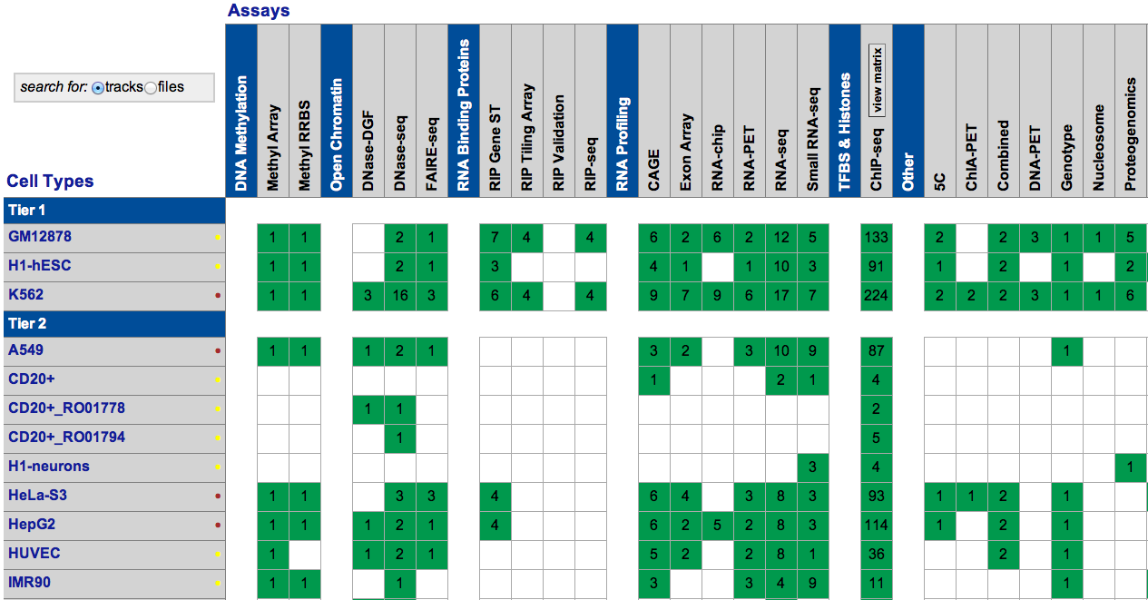
Proyecto ENCODE. Todos los derechos reservados. Este contenido está excluido de nuestro Creativo
Licencia Commons. Para obtener más información, consulte http://ocw.mit.edu/help/faq-fair-use/.
Una de las técnicas más importantes utilizadas fue Chip-seq (inmunoprecipitación de cromatina seguida de secuenciación). El primer paso en un experimento ChIP es apuntar a fragmentos de ADN asociados con una proteína específica. Esto se hace mediante el uso de un anti-cuerpo que se dirige a la proteína específica y se utiliza para inmunoprecipitar el complejo ADN-proteína. El paso final es ensayar el ADN. Esto determinará las secuencias unidas a las proteínas.
Chip-seq tiene varias ventajas sobre las técnicas anteriores (por ejemplo, Chip-chip). Por ejemplo, Chip-seq tiene resolución de un solo nucleótido y su alineabilidad aumenta con la longitud de lectura. Sin embargo, Chip-seq tiene varias desventajas. Los errores de secuenciación tienden a aumentar sustancialmente cerca del final de las lecturas. Además, con un bajo número de lecturas, la sensibilidad y especificidad tienden a disminuir al detectar regiones enriquecidas. Ambos problemas surgen al procesar los datos y muchas de las técnicas computacionales buscan rectificarlo.
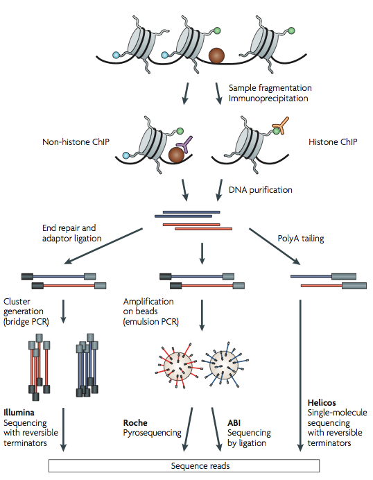
Cortesía de Macmillan Publishers Limited. Usado con permiso.
Fuente: Park, Peter J. “Chip-seq: Ventajas y Desafíos de una
Tecnología de Madurado”. Nature Reviews Genetics 10, núm. 10 (2009): 669-80