

7.1: Coordenadas polares
- Page ID
- 113827
\( \newcommand{\vecs}[1]{\overset { \scriptstyle \rightharpoonup} {\mathbf{#1}} } \)
\( \newcommand{\vecd}[1]{\overset{-\!-\!\rightharpoonup}{\vphantom{a}\smash {#1}}} \)
\( \newcommand{\dsum}{\displaystyle\sum\limits} \)
\( \newcommand{\dint}{\displaystyle\int\limits} \)
\( \newcommand{\dlim}{\displaystyle\lim\limits} \)
\( \newcommand{\id}{\mathrm{id}}\) \( \newcommand{\Span}{\mathrm{span}}\)
( \newcommand{\kernel}{\mathrm{null}\,}\) \( \newcommand{\range}{\mathrm{range}\,}\)
\( \newcommand{\RealPart}{\mathrm{Re}}\) \( \newcommand{\ImaginaryPart}{\mathrm{Im}}\)
\( \newcommand{\Argument}{\mathrm{Arg}}\) \( \newcommand{\norm}[1]{\| #1 \|}\)
\( \newcommand{\inner}[2]{\langle #1, #2 \rangle}\)
\( \newcommand{\Span}{\mathrm{span}}\)
\( \newcommand{\id}{\mathrm{id}}\)
\( \newcommand{\Span}{\mathrm{span}}\)
\( \newcommand{\kernel}{\mathrm{null}\,}\)
\( \newcommand{\range}{\mathrm{range}\,}\)
\( \newcommand{\RealPart}{\mathrm{Re}}\)
\( \newcommand{\ImaginaryPart}{\mathrm{Im}}\)
\( \newcommand{\Argument}{\mathrm{Arg}}\)
\( \newcommand{\norm}[1]{\| #1 \|}\)
\( \newcommand{\inner}[2]{\langle #1, #2 \rangle}\)
\( \newcommand{\Span}{\mathrm{span}}\) \( \newcommand{\AA}{\unicode[.8,0]{x212B}}\)
\( \newcommand{\vectorA}[1]{\vec{#1}} % arrow\)
\( \newcommand{\vectorAt}[1]{\vec{\text{#1}}} % arrow\)
\( \newcommand{\vectorB}[1]{\overset { \scriptstyle \rightharpoonup} {\mathbf{#1}} } \)
\( \newcommand{\vectorC}[1]{\textbf{#1}} \)
\( \newcommand{\vectorD}[1]{\overrightarrow{#1}} \)
\( \newcommand{\vectorDt}[1]{\overrightarrow{\text{#1}}} \)
\( \newcommand{\vectE}[1]{\overset{-\!-\!\rightharpoonup}{\vphantom{a}\smash{\mathbf {#1}}}} \)
\( \newcommand{\vecs}[1]{\overset { \scriptstyle \rightharpoonup} {\mathbf{#1}} } \)
\(\newcommand{\longvect}{\overrightarrow}\)
\( \newcommand{\vecd}[1]{\overset{-\!-\!\rightharpoonup}{\vphantom{a}\smash {#1}}} \)
\(\newcommand{\ket}[1]{\left| #1 \right>}\)
\(\newcommand{\bra}[1]{\left< #1 \right|}\)
\(\newcommand{\braket}[2]{\left< #1 \vphantom{#2} \right| \left. #2 \vphantom{#1} \right>}\)
\(\newcommand{\braopket}[3]{\left< #1 \vphantom{#2}\vphantom{#3} \right| #2 \vphantom{#1}\vphantom{#3} \left| #3 \vphantom{#1}\vphantom{#2} \right>}\)
\(\newcommand{\qmvec}[1]{\mathbf{\vec{#1}}}\)
\(\newcommand{\op}[1]{\hat{\mathbf{#1}}}\)
\(\newcommand{\expect}[1]{\langle #1 \rangle}\)
\(\newcommand{\dfn}[1]{\emph{\textbf{#1}}}\)
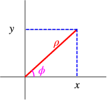
Las coordenadas polares en dos dimensiones se definen\[\begin{aligned} x = \rho\cos\phi, y= \rho\sin\phi,\\ \rho = \sqrt{x^2+y^2}, \phi = \arctan(y/x),\end{aligned} \nonumber \] como se indica esquemáticamente en la Fig. \(\PageIndex{1}\).
Usando la regla de la cadena encontramos
\[\begin{aligned} \frac{\partial}{\partial x}{~} &= \frac{\partial \rho}{\partial x}\frac{\partial}{\partial \rho}{~}+\frac{\partial \phi}{\partial x}\frac{\partial}{\partial \phi}{~}\nonumber\\ &= \frac{x}{\rho}\frac{\partial}{\partial \rho}{~}-\frac{y}{\rho^2}\frac{\partial}{\partial \phi}{~}\nonumber\\ &= \cos\phi\frac{\partial}{\partial \rho}{~}-\frac{\sin\phi}{\rho}\frac{\partial}{\partial \phi}{~},\\ \frac{\partial}{\partial y}{~} &= \frac{\partial \rho}{\partial y}\frac{\partial}{\partial \rho}{~}+\frac{\partial \phi}{\partial y}\frac{\partial}{\partial \phi}{~}\nonumber\\ &= \frac{y}{\rho}\frac{\partial}{\partial \rho} {~}+\frac{x}{\rho^2}\frac{\partial}{\partial \phi}{~}\nonumber\\ &= \sin\phi\frac{\partial}{\partial \rho}{~}+\frac{\cos\phi}{\rho}\frac{\partial}{\partial \phi}{~},\end{aligned} \nonumber \]Podemos escribir\[\begin{aligned} {\nabla} &= {\hat{e}}_\rho \frac{\partial}{\partial \rho}{~}+\hat{e}_\phi \frac{1}{\rho} \frac{\partial}{\partial \phi}{~}\end{aligned} \nonumber \]
donde los vectores unitarios
\[\begin{aligned} \hat{e}_\rho &= (\cos\phi,\sin\phi), \nonumber\\ \hat{e}_\phi &= (-\sin\phi,\cos\phi), \end{aligned} \nonumber \]son un conjunto ortonormal. Decimos que las coordenadas circulares son ortogonales.
Ahora podemos usar esto para evaluar\(\nabla^2\),
\[\begin{aligned} \nabla^2 &= \cos^2\phi\frac{\partial^2}{\partial \rho^2}{~} + \frac{\sin\phi\cos\phi}{\rho^2}\frac{\partial}{\partial \phi} {~} +\frac{\sin^2\phi}{\rho}\frac{\partial}{\partial \rho} {~} + \frac{\sin^2\phi}{\rho^2}\frac{\partial^2}{\partial \phi^2} {~} + \frac{\sin\phi\cos\phi}{\rho^2} \frac{\partial}{\partial \phi} {~}\nonumber\\ &\space\space\space+\sin^2\phi\frac{\partial^2}{\partial \rho^2} {~}-\frac{\sin\phi\cos\phi}{\rho^2}\frac{\partial}{\partial \phi} {~} +\frac{\cos^2\phi}{\rho}\frac{\partial}{\partial \rho} {~} + \frac{\cos^2\phi}{\rho^2}\frac{\partial^2}{\partial \phi^2} {~} - \frac{\sin\phi\cos\phi}{\rho^2} \frac{\partial}{\partial \phi}{~}\\ &=\frac{\partial^2}{\partial \rho^2} {~} +\frac{1}{\rho}\frac{\partial}{\partial \rho}{~} + \frac{1}{\rho^2}\frac{\partial^2}{\partial \phi^2} {~}\nonumber\\ &=\frac{1}{\rho}\frac{\partial}{\partial \rho} {~} \left(\rho\frac{\partial}{\partial \rho} {~}\right) +\frac{1}{\rho^2}\frac{\partial^2}{\partial \phi^2} {~}.\nonumber\\\end{aligned} \nonumber \]
Una relación útil final es la integración sobre estas coordenadas.
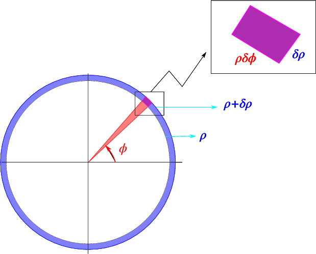
Como se indica esquemáticamente en la Fig. \(\PageIndex{2}\), la superficie relacionada con un cambio\(\rho \rightarrow \rho + \delta \rho\),\(\phi \rightarrow \phi+\delta\phi\) es\(\rho \delta \rho \delta\phi\). Esto nos lleva a la conclusión de que una integral sobre\(x,y\) puede reescribirse como\[\int_V f(x,y) dx dy = \int_V f(\rho\cos\phi,\rho\sin\phi) \rho \,d\rho\, d\phi \nonumber \]