

12.9: Trigonometría hiperbólica
- Page ID
- 114373
\( \newcommand{\vecs}[1]{\overset { \scriptstyle \rightharpoonup} {\mathbf{#1}} } \)
\( \newcommand{\vecd}[1]{\overset{-\!-\!\rightharpoonup}{\vphantom{a}\smash {#1}}} \)
\( \newcommand{\dsum}{\displaystyle\sum\limits} \)
\( \newcommand{\dint}{\displaystyle\int\limits} \)
\( \newcommand{\dlim}{\displaystyle\lim\limits} \)
\( \newcommand{\id}{\mathrm{id}}\) \( \newcommand{\Span}{\mathrm{span}}\)
( \newcommand{\kernel}{\mathrm{null}\,}\) \( \newcommand{\range}{\mathrm{range}\,}\)
\( \newcommand{\RealPart}{\mathrm{Re}}\) \( \newcommand{\ImaginaryPart}{\mathrm{Im}}\)
\( \newcommand{\Argument}{\mathrm{Arg}}\) \( \newcommand{\norm}[1]{\| #1 \|}\)
\( \newcommand{\inner}[2]{\langle #1, #2 \rangle}\)
\( \newcommand{\Span}{\mathrm{span}}\)
\( \newcommand{\id}{\mathrm{id}}\)
\( \newcommand{\Span}{\mathrm{span}}\)
\( \newcommand{\kernel}{\mathrm{null}\,}\)
\( \newcommand{\range}{\mathrm{range}\,}\)
\( \newcommand{\RealPart}{\mathrm{Re}}\)
\( \newcommand{\ImaginaryPart}{\mathrm{Im}}\)
\( \newcommand{\Argument}{\mathrm{Arg}}\)
\( \newcommand{\norm}[1]{\| #1 \|}\)
\( \newcommand{\inner}[2]{\langle #1, #2 \rangle}\)
\( \newcommand{\Span}{\mathrm{span}}\) \( \newcommand{\AA}{\unicode[.8,0]{x212B}}\)
\( \newcommand{\vectorA}[1]{\vec{#1}} % arrow\)
\( \newcommand{\vectorAt}[1]{\vec{\text{#1}}} % arrow\)
\( \newcommand{\vectorB}[1]{\overset { \scriptstyle \rightharpoonup} {\mathbf{#1}} } \)
\( \newcommand{\vectorC}[1]{\textbf{#1}} \)
\( \newcommand{\vectorD}[1]{\overrightarrow{#1}} \)
\( \newcommand{\vectorDt}[1]{\overrightarrow{\text{#1}}} \)
\( \newcommand{\vectE}[1]{\overset{-\!-\!\rightharpoonup}{\vphantom{a}\smash{\mathbf {#1}}}} \)
\( \newcommand{\vecs}[1]{\overset { \scriptstyle \rightharpoonup} {\mathbf{#1}} } \)
\(\newcommand{\longvect}{\overrightarrow}\)
\( \newcommand{\vecd}[1]{\overset{-\!-\!\rightharpoonup}{\vphantom{a}\smash {#1}}} \)
\(\newcommand{\ket}[1]{\left| #1 \right>}\)
\(\newcommand{\bra}[1]{\left< #1 \right|}\)
\(\newcommand{\braket}[2]{\left< #1 \vphantom{#2} \right| \left. #2 \vphantom{#1} \right>}\)
\(\newcommand{\braopket}[3]{\left< #1 \vphantom{#2}\vphantom{#3} \right| #2 \vphantom{#1}\vphantom{#3} \left| #3 \vphantom{#1}\vphantom{#2} \right>}\)
\(\newcommand{\qmvec}[1]{\mathbf{\vec{#1}}}\)
\(\newcommand{\op}[1]{\hat{\mathbf{#1}}}\)
\(\newcommand{\expect}[1]{\langle #1 \rangle}\)
\(\newcommand{\dfn}[1]{\emph{\textbf{#1}}}\)
En esta sección damos fórmulas para h-distancia usando funciones hiperbólicas. Una de estas fórmulas se utilizará en la prueba del teorema hiperbólico de Pitágoras (Teorema 13.6.1).
Recordemos que\(\cosh\)\(\sinh\), y\(\tanh\) denotan coseno hiperbólico, seno hiperbólico y tangente hiperbólica; es decir, las funciones definidas por
\(\cosh x := \dfrac{e^x + e^{-x}}{2}\),\(\sinh x := \dfrac{e^x - e^{-x}}{2}\),
\(\tanh x := \dfrac{\sinh x}{\cosh x}.\)
Estas funciones hiperbólicas son análogas a seno y coseno y tangente.
Demostrar las siguientes identidades:
\(\cosh' x=\sinh x\);\(\sinh'x=\cosh x\);\((\cosh x)^2-(\sinh x)^2=1.\)
Las identidades
\(\cosh (2 \cdot x) = (\cosh x)^2 + (\sinh x)^2\)y\(\sinh (2 \cdot x) = 2 \cdot \sinh x \cdot \cosh x\)
mantener por cualquier valor real\(x\).
- Prueba
-
\(\begin{array} {rcl} {(\sinh x)^2 + (\cosh x)^2} & = & {(\dfrac{e^x - e^{-x}}{2})^2 + (\dfrac{e^x + e^{-x}}{2})^2 =} \\ {} & = & {\dfrac{e^{2 \cdot x} + e^{-2 \cdot x}}{2} =} \\ {} & = & {\cosh (2 \cdot x);} \end{array}\)
\(\begin{array} {rcl} {2 \cdot \sinh x \cdot cosh x} & = & {2 \cdot (\dfrac{e^x - e^{-x}}{2}) \cdot (\dfrac{e^x + e^{-x}}{2})} \\ {} & = & {\dfrac{e^{2 \cdot x} - e^{-2 \cdot x}}{2}} \\ {} & = & {\cosh (2 \cdot x).} \end{array}\)
Dejar\(P\) y\(Q\) ser dos h-poins distintos del centro de absoluto. Denotar por\(P'\) y\(Q'\) las inversas de\(P\) y\(Q\) en lo absoluto.
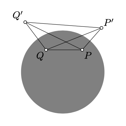
(a)\(\cosh [\dfrac{1}{2} \cdot PQ_h] = \sqrt{\dfrac{PQ' \cdot P'Q}{PP' \cdot QQ'}};\)
b)\(\sinh [\dfrac{1}{2} \cdot PQ_h] = \sqrt{\dfrac{PQ \cdot P'Q'}{PP' \cdot QQ'}};\)
c)\(\tanh [\dfrac{1}{2} \cdot PQ_h] = \sqrt{\dfrac{PQ \cdot P'Q'}{PQ' \cdot P'Q}};\)
d)\(\cosh PQ_h = \dfrac{PQ \cdot P'Q' + PQ' \cdot P'Q}{PP' \cdot QQ'}\).
- Insinuación
-
Por Corolario 10.6.1 y Teorema 10.2.1, los lados derechos en las identidades sobreviven bajo una inversión en un círculo perpendicular a lo absoluto.
Como de costumbre suponemos que el absoluto es un círculo unitario. Supongamos que\(O\) denota el punto medio h de\([PQ]_h\). Por la observación principal (Teorema 12.3.1) podemos suponer que\(O\) es el centro de lo absoluto. En este caso también\(O\) es el punto medio euclidiano de\([P Q]\). (En cambio, podemos movernos\(Q\) al centro de lo absoluto. En este caso las derivaciones son más sencillas. Pero desde entonces\(Q'Q = Q'P = QP = \infty\), uno tiene que justificar eso\(\dfrac{\infty}{\infty} = 1\) cada vez.)
Set\(a = OP = OQ\); en este caso tenemos
\(\begin{array} {rcl} {PQ} & = & {2 \cdot a,} \\ {P'Q'} & = & {2 \cdot \dfrac{1}{a},} \end{array}\)\(\begin{array} {l} {PP' = QQ' = \dfrac{1}{a} - a,} \\ {PQ' = QP' = \dfrac{1}{a} + a.} \end{array}\)
y
\(PQ_h = \ln \dfrac{(1 + a)^2}{(1 - a)^2} = 2 \cdot \ln \dfrac{1 + a}{1 - a}.\)
Por lo tanto
\(\begin{array} {rcl} {\cosh [\dfrac{1}{2} \cdot PQ_h]} & = & {\dfrac{1}{2} \cdot (\dfrac{1 + a}{1 - a} + \dfrac{1 - a}{1 + a})=} \\ {} & = & {\dfrac{1 + a^2}{1 - a^2};} \end{array}\)\(\begin{array} {rcl} {\sqrt{\dfrac{PQ' \cdot P'Q}{PP' \cdot QQ'}}} & = & {\dfrac{\dfrac{1}{a} + a}{\dfrac{1}{a} - a} =} \\ {} & = & {\dfrac{1 + a^2}{1 - a^2}.} \end{array}\)
De ahí que siga la parte a). Del mismo modo,
\(\begin{array} {rcl} {\sinh [\dfrac{1}{2} \cdot PQ_h]} & = & {\dfrac{1}{2} \cdot (\dfrac{1 + a}{1 - a} - \dfrac{1 - a}{1 + a}) =} \\ {} & = & {\dfrac{2 \cdot a}{1 - a^2};} \end{array}\)\(\begin{array} {rcl} {\sqrt{\dfrac{PQ \cdot P'Q'}{PP' \cdot QQ'}}} & = & {\dfrac{2}{\dfrac{1}{a} - a} =} \\ {} & = & {\dfrac{2 \cdot a}{1 - a^2}.} \end{array}\)
De ahí que siga la parte b).
Las partes (c) y (d) siguen de (a), (b), la definición de tangente hiperbólica, y la identidad de doble argumento para el coseno hiperbólico, ver Teorema\(\PageIndex{1}\).