

4.11: Funciones de definición a trozos
- Page ID
- 112500

\( \newcommand{\vecs}[1]{\overset { \scriptstyle \rightharpoonup} {\mathbf{#1}} } \)
\( \newcommand{\vecd}[1]{\overset{-\!-\!\rightharpoonup}{\vphantom{a}\smash {#1}}} \)
\( \newcommand{\dsum}{\displaystyle\sum\limits} \)
\( \newcommand{\dint}{\displaystyle\int\limits} \)
\( \newcommand{\dlim}{\displaystyle\lim\limits} \)
\( \newcommand{\id}{\mathrm{id}}\) \( \newcommand{\Span}{\mathrm{span}}\)
( \newcommand{\kernel}{\mathrm{null}\,}\) \( \newcommand{\range}{\mathrm{range}\,}\)
\( \newcommand{\RealPart}{\mathrm{Re}}\) \( \newcommand{\ImaginaryPart}{\mathrm{Im}}\)
\( \newcommand{\Argument}{\mathrm{Arg}}\) \( \newcommand{\norm}[1]{\| #1 \|}\)
\( \newcommand{\inner}[2]{\langle #1, #2 \rangle}\)
\( \newcommand{\Span}{\mathrm{span}}\)
\( \newcommand{\id}{\mathrm{id}}\)
\( \newcommand{\Span}{\mathrm{span}}\)
\( \newcommand{\kernel}{\mathrm{null}\,}\)
\( \newcommand{\range}{\mathrm{range}\,}\)
\( \newcommand{\RealPart}{\mathrm{Re}}\)
\( \newcommand{\ImaginaryPart}{\mathrm{Im}}\)
\( \newcommand{\Argument}{\mathrm{Arg}}\)
\( \newcommand{\norm}[1]{\| #1 \|}\)
\( \newcommand{\inner}[2]{\langle #1, #2 \rangle}\)
\( \newcommand{\Span}{\mathrm{span}}\) \( \newcommand{\AA}{\unicode[.8,0]{x212B}}\)
\( \newcommand{\vectorA}[1]{\vec{#1}} % arrow\)
\( \newcommand{\vectorAt}[1]{\vec{\text{#1}}} % arrow\)
\( \newcommand{\vectorB}[1]{\overset { \scriptstyle \rightharpoonup} {\mathbf{#1}} } \)
\( \newcommand{\vectorC}[1]{\textbf{#1}} \)
\( \newcommand{\vectorD}[1]{\overrightarrow{#1}} \)
\( \newcommand{\vectorDt}[1]{\overrightarrow{\text{#1}}} \)
\( \newcommand{\vectE}[1]{\overset{-\!-\!\rightharpoonup}{\vphantom{a}\smash{\mathbf {#1}}}} \)
\( \newcommand{\vecs}[1]{\overset { \scriptstyle \rightharpoonup} {\mathbf{#1}} } \)
\(\newcommand{\longvect}{\overrightarrow}\)
\( \newcommand{\vecd}[1]{\overset{-\!-\!\rightharpoonup}{\vphantom{a}\smash {#1}}} \)
\(\newcommand{\ket}[1]{\left| #1 \right>}\)
\(\newcommand{\bra}[1]{\left< #1 \right|}\)
\(\newcommand{\braket}[2]{\left< #1 \vphantom{#2} \right| \left. #2 \vphantom{#1} \right>}\)
\(\newcommand{\braopket}[3]{\left< #1 \vphantom{#2}\vphantom{#3} \right| #2 \vphantom{#1}\vphantom{#3} \left| #3 \vphantom{#1}\vphantom{#2} \right>}\)
\(\newcommand{\qmvec}[1]{\mathbf{\vec{#1}}}\)
\(\newcommand{\op}[1]{\hat{\mathbf{#1}}}\)
\(\newcommand{\expect}[1]{\langle #1 \rangle}\)
\(\newcommand{\dfn}[1]{\emph{\textbf{#1}}}\)
Las funciones definidas por partes son funciones que se definen usando diferentes ecuaciones para diferentes partes del dominio.
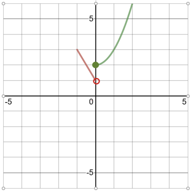
Evalúe la siguiente función definida por partes para los valores dados de\(x\), y grafique la función:
\(f(x) = \left\{\begin{array}{cc}−2x + 1 & −1 \leq x < 0 \\ x^2 + 2 &0 \leq x \leq 2\end{array} \right.\)
Solución
Para graficar esta función, haz una tabla de soluciones:
|
Tabla de soluciones para\(f(x) = −2x + 1 \) Dominio\(−1 \leq x < 0\) |
|
| \(x\) | \(f(x)\) |
| -1 | 3 |
| 0 | 1 (círculo abierto aquí, 0 no en el dominio) |
|
Tabla de soluciones para\(f(x) = x^2 + 2\) Dominio\(0 \leq x \leq 2\) |
|
| \(x\) | \(f(x)\) |
| 0 | 2 |
| 1 | 3 |
| 2 | 6 |
Evalúe la siguiente función definida por partes para los valores dados de\(x\), y grafique la función:
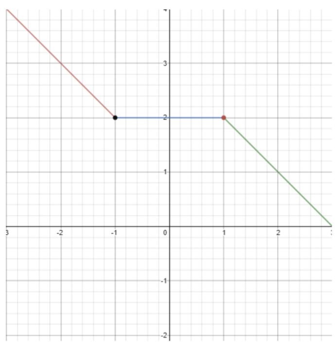
\(f(x) = \left\{\begin{array}{cc} −x + 1 &x \leq −1 \\ 2 & −1 < x \leq 1 \\ −x + 3 &x > 1 \end{array}\right.\)
Solución
Para graficar esta función, una vez más haga una tabla de soluciones:
|
Tabla de soluciones para\(f(x) = −x + 1\) Dominio\(x \leq −1\) |
|
| \(x\) | \(f(x)\) |
| -3 | 4 |
| -2 | 3 |
| -1 | 2 (círculo cerrado aquí, -1 está en el dominio) |
|
Tabla de soluciones para\(f(x) = 2\) Dominio\(−1 < x \leq 1\) |
|
| \(x\) | \(f(x)\) |
| -1 | 2 (círculo abierto rellenado por la función anterior, -1 no en el dominio) |
| 0 | 2 |
| 1 | 2 (círculo cerrado aquí, 1 está en el dominio) |
|
Tabla de soluciones para\(f(x) = −x + 3\) Dominio\(x > 1\) |
|
| \(x\) | \(f(x)\) |
| 1 | 2 (círculo abierto rellenado por la función anterior, 1 no en el dominio) |
| 2 | 1 |
| 3 | 0 |
Evaluar las siguientes funciones definidas por partes para los valores dados de x, y graficar las funciones:.
- \ (f (x) =\ left\ {\ begin {array} {cc}
x & x<0\\
2 x+1 &x\ geq 0
\ end {array}\ right.\) - \(g(x) = \left\{\begin{array}{cc} 4 − x& x < 2\\ 2x − 2 &x \geq 2 \end{array} \right.\)
- \(h(x) = \left\{\begin{array}{cc} −x − 1 & x < −1 \\ 0& −1 \leq x \leq 1 \\ x + 1 & x > 1 \end{array} \right.\)
- \(g(x) = \left\{\begin{array}{cc} 6 & −8 \leq x < −4 \\ 3 &−4 \leq x \leq 5 \end{array}\right.\)
- \(f(x) = \left\{\begin{array}{cc} −x + 1 & −1 \leq x < 1 \\ \sqrt{x − 1 } &1 \leq x \leq 5\end{array}\right.\)