2.3: Circuitos paralelos
- Page ID
- 152802

\( \newcommand{\vecs}[1]{\overset { \scriptstyle \rightharpoonup} {\mathbf{#1}} } \)
\( \newcommand{\vecd}[1]{\overset{-\!-\!\rightharpoonup}{\vphantom{a}\smash {#1}}} \)
\( \newcommand{\dsum}{\displaystyle\sum\limits} \)
\( \newcommand{\dint}{\displaystyle\int\limits} \)
\( \newcommand{\dlim}{\displaystyle\lim\limits} \)
\( \newcommand{\id}{\mathrm{id}}\) \( \newcommand{\Span}{\mathrm{span}}\)
( \newcommand{\kernel}{\mathrm{null}\,}\) \( \newcommand{\range}{\mathrm{range}\,}\)
\( \newcommand{\RealPart}{\mathrm{Re}}\) \( \newcommand{\ImaginaryPart}{\mathrm{Im}}\)
\( \newcommand{\Argument}{\mathrm{Arg}}\) \( \newcommand{\norm}[1]{\| #1 \|}\)
\( \newcommand{\inner}[2]{\langle #1, #2 \rangle}\)
\( \newcommand{\Span}{\mathrm{span}}\)
\( \newcommand{\id}{\mathrm{id}}\)
\( \newcommand{\Span}{\mathrm{span}}\)
\( \newcommand{\kernel}{\mathrm{null}\,}\)
\( \newcommand{\range}{\mathrm{range}\,}\)
\( \newcommand{\RealPart}{\mathrm{Re}}\)
\( \newcommand{\ImaginaryPart}{\mathrm{Im}}\)
\( \newcommand{\Argument}{\mathrm{Arg}}\)
\( \newcommand{\norm}[1]{\| #1 \|}\)
\( \newcommand{\inner}[2]{\langle #1, #2 \rangle}\)
\( \newcommand{\Span}{\mathrm{span}}\) \( \newcommand{\AA}{\unicode[.8,0]{x212B}}\)
\( \newcommand{\vectorA}[1]{\vec{#1}} % arrow\)
\( \newcommand{\vectorAt}[1]{\vec{\text{#1}}} % arrow\)
\( \newcommand{\vectorB}[1]{\overset { \scriptstyle \rightharpoonup} {\mathbf{#1}} } \)
\( \newcommand{\vectorC}[1]{\textbf{#1}} \)
\( \newcommand{\vectorD}[1]{\overrightarrow{#1}} \)
\( \newcommand{\vectorDt}[1]{\overrightarrow{\text{#1}}} \)
\( \newcommand{\vectE}[1]{\overset{-\!-\!\rightharpoonup}{\vphantom{a}\smash{\mathbf {#1}}}} \)
\( \newcommand{\vecs}[1]{\overset { \scriptstyle \rightharpoonup} {\mathbf{#1}} } \)
\(\newcommand{\longvect}{\overrightarrow}\)
\( \newcommand{\vecd}[1]{\overset{-\!-\!\rightharpoonup}{\vphantom{a}\smash {#1}}} \)
\(\newcommand{\ket}[1]{\left| #1 \right>}\)
\(\newcommand{\bra}[1]{\left< #1 \right|}\)
\(\newcommand{\braket}[2]{\left< #1 \vphantom{#2} \right| \left. #2 \vphantom{#1} \right>}\)
\(\newcommand{\braopket}[3]{\left< #1 \vphantom{#2}\vphantom{#3} \right| #2 \vphantom{#1}\vphantom{#3} \left| #3 \vphantom{#1}\vphantom{#2} \right>}\)
\(\newcommand{\qmvec}[1]{\mathbf{\vec{#1}}}\)
\(\newcommand{\op}[1]{\hat{\mathbf{#1}}}\)
\(\newcommand{\expect}[1]{\langle #1 \rangle}\)
\(\newcommand{\dfn}[1]{\emph{\textbf{#1}}}\)
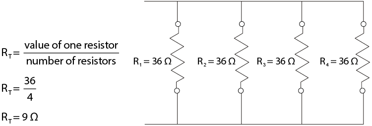
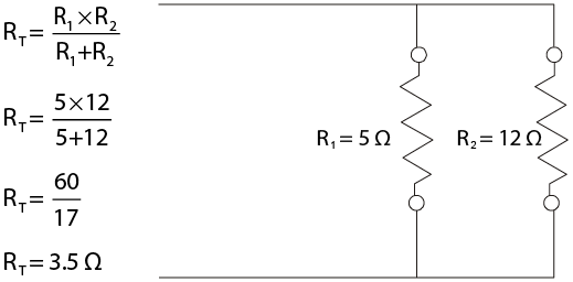
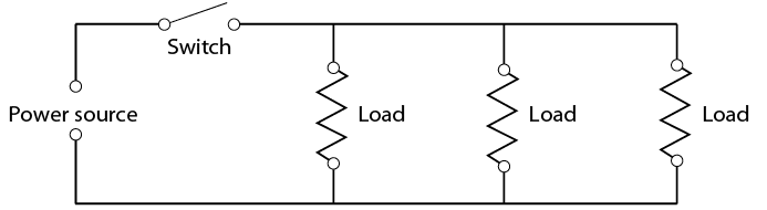
El circuito paralelo (Figura\(\PageIndex{1}\)) tiene características completamente diferentes. En un circuito paralelo, dos o más cargas están conectadas una al lado de la otra y son controladas por uno o más interruptores. Las diferentes cargas pueden tener cada una su propio interruptor, pero la diferencia principal es que cada una de las cargas tiene acceso a la misma cantidad de voltaje y puede operar independientemente de las demás. Hay más de un camino por el que puede fluir la corriente.
saf
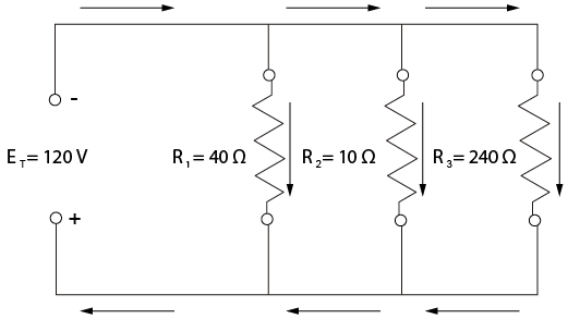
\[\begin{array}{l}{\mathrm{I}_{1}=\frac{\mathrm{E}_{1}}{\mathrm{R}_{1}}=\frac{120}{40}=3 \mathrm{amps}} \\ {\mathrm{I}_{2}=\frac{\mathrm{E}_{2}}{\mathrm{R}_{2}}=\frac{120}{10}=12 \mathrm{amps}} \\ {\mathrm{I}_{3}=\frac{\mathrm{E}_{3}}{\mathrm{R}_{3}}=\frac{120}{240}=0.5 \mathrm{amp}}\end{array}\]
\[R_{T}=\frac{E_{T}}{I_{T}}=\frac{120}{15.5}=7.7 \text { ohms }\]
\[R_{T}=\frac{1}{\frac{1}{R_{1}}+\frac{1}{R_{2}}+\frac{1}{R_{3}} \ldots}\]
\[\begin{aligned} R_{T}=& \frac{1}{\frac{1}{40}+\frac{1}{10}+\frac{1}{240}}=7.7 \text { ohms } \\ R_{T}=& \frac{1}{\frac{6}{240}+\frac{24}{240}+\frac{1}{240}} \\ R_{T}=& \frac{\frac{240}{240}}{31} \\ R_{T}=& 7.7 \text { ohms } \end{aligned}\]