8.1.5: Tablas para encontrar límites

Tablas para encontrar límites

Las calculadoras como la TI-84 tienen una vista de tabla que le permite hacer conjeturas extremadamente educadas sobre cuál será el límite de una función en un punto específico, incluso si la función no está realmente definida en ese punto.

¿Cómo podrías usar una tabla para calcular el siguiente límite?

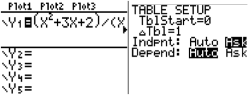
\(\ \lim _{x \rightarrow-1} \frac{x^{2}+3 x+2}{x+1}\)

---

Uso de tablas para encontrar límites

Si te dieran la siguiente información organizada en una tabla, ¿cómo rellenarías la columna central?

3.9	3.99	3.999		4.001	4.01	4.1
12.25	12.01	12.00001		11.99999	11.99	11.75

Sería lógico ver la simetría y notar cómo la fila superior se acerca al número 4 desde la izquierda y la derecha. También sería lógico notar cómo la fila inferior se acerca al número 12 desde la izquierda y la derecha. Esto le llevaría a la conclusión de que el límite de la función representada por esta tabla es 12 ya que la fila superior se acerca a 4. No importaría si el valor en 4 estaba indefinido o definido para ser otro número como 17, el patrón te dice que el límite en 4 es 12.

El uso de tablas para ayudar a evaluar los límites numéricamente requiere este tipo de lógica. Numéricamente es un término utilizado para describir una de varias representaciones diferentes en matemáticas. Se refiere a tablas donde los números reales son visibles.

Para estimar el límite\(\ \lim _{x \rightarrow 2} \frac{x-2}{x^{2}-x-2}\), complete la tabla:

x	1.9	1.99	1.999	2.001	2.01	2.1
f (x)

Si bien no es necesario utilizar la función de tabla en la calculadora, es muy eficiente.

Para usar una tabla en su calculadora para evaluar un límite:

1. Ingresa la función en la pantalla y=
2. Ir a la configuración de la tabla y resaltar “preguntar” para la variable independiente
3. Ir a la tabla e introducir valores cercanos al número que x se acerca

Otra opción es sustituir los\(\ x\) valores dados en la expresión\(\ \frac{x-2}{x^{2}-x-2}\) y registrar sus resultados. De cualquier manera, la tabla terminada es la siguiente.

x	1.9	1.99	1.999	2.001	2.01	2.1
f (x)	0.34483	0.33445	0.33344	0.33322	0.33223	0.32258

La evidencia sugiere que el límite es\(\ \frac{1}{3}\).

---

Ejemplos

Ejemplo 1

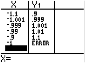
Antes, se le pidió que encontrara el límite de\(\ \lim _{x \rightarrow-1} \frac{x^{2}+3 x+2}{x+1}\).

Solución

Cuando ingresas valores cercanos a -1 en la tabla obtienes\(\ y\) valores que están cada vez más cerca del número 1. Esto implica que el límite a medida que\(\ x\) se acerca a -1 es 1. Observe que cuando evalúa la función en -1, la calculadora produce un error. Esto debería llevarte a la conclusión de que si bien la función no está definida en\(\ x=−1\), el límite sí existe.

Ejemplo 2

Completa la tabla y usa el resultado para estimar el límite.

\(\ \lim _{x \rightarrow 2} \frac{x-2}{x^{2}-4}\)

x	1.9	1.99	1.999	2.001	2.01	2.1
f (x)

Solución

Puedes engañar a la calculadora para que dé una respuesta muy exacta escribiendo 1.9999999999 porque entonces la calculadora redondea en lugar de producir un error.

x	1.9	1.99	1.999	2.001	2.01	2.1
f (x)	0.25641	0.25063	0.25006	0.24994	0.24938	0.2439

La evidencia sugiere que el límite es\(\ \frac{1}{4}\).

Ejemplo 3

Completa la tabla y usa el resultado para estimar el límite.

\(\ \lim _{x \rightarrow 0} \frac{\sqrt{x+3}-\sqrt{3}}{x}\)

x	-0.1	-0.01	-0.001	0.001	0.01	0.1
f (x)

Solución

x	-0.1	-0.01	-0.001	0.001	0.01	0.1
f (x)	0.29112	0.28892	0.2887	0.28865	0.28843	0.28631

La evidencia sugiere que el límite es un número entre 0.2887 y 0.28865. Cuando aprendas a encontrar el límite analíticamente, sabrás que el límite exacto es\(\ \frac{1}{2} \cdot 3 \frac{1}{2} \approx 0.2886751346\).

Ejemplo 4

Grafica la siguiente función y el uso de una tabla para verificar el límite a medida que se\(\ x\) acerca a 1.

\(\ f(x)=\frac{x^{3}-1}{x-1}, x \neq 1\)

Solución

\(\ \lim _{x \rightarrow 1} f(x)=3\). Esto se debe a que cuando factoriza el numerador y cancela factores comunes, la función se convierte en una cuadrática con un agujero en el punto\(\ (1, 3)\).

Se puede verificar el límite en la tabla.

x	f (x)
.75	2.3125
.9	2.71
.99	2.9701
.999	2.997
1	Error
1.001	3.003
1.01	3.0301
1.1	3.31
1.25	3.8125

Ejemplo 5

Estimar el límite numéricamente.

\(\ \lim _{x \rightarrow 0} \frac{\left[\frac{4}{x+2}\right]-2}{x}\)

Solución

x	-0.1	-0.01	-0.001	0.001	0.01	0.1
f (x)	0.20526	0.02005	0.002	-0.002	-0.02	-0.1952

\(\ \lim _{x \rightarrow 0} f(x)=0\)

---

Revisar

Estimar numéricamente los siguientes límites.

1. \(\ \lim _{x \rightarrow 5} \frac{x^{2}-25}{x-5}\)
2. \(\ \lim _{x \rightarrow-1} \frac{x^{2}-3 x-4}{x+1}\)
3. \(\ \lim _{x \rightarrow 2} \frac{x^{3}-5 x^{2}+2 x-4}{x^{2}-3 x+2}\)
4. \(\ \lim _{x \rightarrow 0} \frac{\sqrt{x+2}-\sqrt{2}}{x}\)
5. \(\ \lim _{x \rightarrow 3}\left(\frac{1}{x-3}-\frac{9}{x^{2}-9}\right)\)
6. \(\ \lim _{x \rightarrow 2} \frac{x^{2}+5 x-14}{x-2}\)
7. \(\ \lim _{x \rightarrow 1} \frac{x^{2}-8 x+7}{x-1}\)
8. \(\ \lim _{x \rightarrow 0} \frac{\sqrt{x+5}-\sqrt{5}}{x}\)
9. \(\ \lim _{x \rightarrow 9} \frac{\sqrt{x}-3}{x-9}\)
10. \(\ \lim _{x \rightarrow 0} \frac{x^{2}+5 x}{x}\)
11. \(\ \lim _{x \rightarrow-3} \frac{x^{2}-9}{x+3}\)
12. \(\ \lim _{x \rightarrow 4} \frac{\sqrt{x}-2}{x-4}\)
13. \(\ \lim _{x \rightarrow 2} \frac{\sqrt{x+3}-2}{x-1}\)
14. \(\ \lim _{x \rightarrow 5} \frac{x^{2}-25}{x^{3}-125}\)
15. \(\ \lim _{x \rightarrow-1} \frac{x-2}{x+1}\)

---

Reseña (Respuestas)

Para ver las respuestas de Revisar, abra este archivo PDF y busque la sección 14.3.

---

El vocabulario

Término	Definición
límite	Un límite es el valor que la salida de una función se acerca a medida que la entrada de la función se acerca a un valor dado.
numéricamente	Numéricamente es un término utilizado para describir una de varias representaciones diferentes en matemáticas. Se refiere a tablas donde los números reales son visibles.

---

Atribuciones de imagen

1. [Figura 1]
   Crédito: Fundación CK-12
   Licencia: CC BY-SA