5.2.5: Curvas polares equivalentes

Última actualización
Guardar como PDF

Page ID: 107755

\( \newcommand{\vecs}[1]{\overset { \scriptstyle \rightharpoonup} {\mathbf{#1}} } \) \( \newcommand{\vecd}[1]{\overset{-\!-\!\rightharpoonup}{\vphantom{a}\smash {#1}}} \)\(\newcommand{\id}{\mathrm{id}}\) \( \newcommand{\Span}{\mathrm{span}}\) \( \newcommand{\kernel}{\mathrm{null}\,}\) \( \newcommand{\range}{\mathrm{range}\,}\) \( \newcommand{\RealPart}{\mathrm{Re}}\) \( \newcommand{\ImaginaryPart}{\mathrm{Im}}\) \( \newcommand{\Argument}{\mathrm{Arg}}\) \( \newcommand{\norm}[1]{\| #1 \|}\) \( \newcommand{\inner}[2]{\langle #1, #2 \rangle}\) \( \newcommand{\Span}{\mathrm{span}}\) \(\newcommand{\id}{\mathrm{id}}\) \( \newcommand{\Span}{\mathrm{span}}\) \( \newcommand{\kernel}{\mathrm{null}\,}\) \( \newcommand{\range}{\mathrm{range}\,}\) \( \newcommand{\RealPart}{\mathrm{Re}}\) \( \newcommand{\ImaginaryPart}{\mathrm{Im}}\) \( \newcommand{\Argument}{\mathrm{Arg}}\) \( \newcommand{\norm}[1]{\| #1 \|}\) \( \newcommand{\inner}[2]{\langle #1, #2 \rangle}\) \( \newcommand{\Span}{\mathrm{span}}\)\(\newcommand{\AA}{\unicode[.8,0]{x212B}}\)

Mientras trabajas en un problema en la clase de matemáticas, obtienes una solución con cierta ecuación. En este caso, tu solución es\(3+2\cos (\theta )\). Tu amigo se acerca y te dice que piensa que ha resuelto el problema. No obstante, cuando te muestra su papel, su ecuación se ve diferente a la tuya. Su solución es\(−3+2\cos (−\theta )\). ¿Hay alguna manera de determinar si las dos ecuaciones son equivalentes?

La expresión “lo mismo solo diferente” entra en juego en esta sección. Graficaremos dos ecuaciones polares distintas que producirán dos gráficas equivalentes. Usa tu calculadora gráfica y crea estas curvas a medida que se presentan las ecuaciones.

En alguna otra sección, se generaron gráficas de un limaçon, un limaçon hoyuelos, un limaçon en bucle y un cardioide. Todos estos eran de la forma\(r=a\pm b\sin \theta \) o\(r=a\pm b\cos \theta \). La forma más fácil de ver qué ecuaciones polares producen curvas equivalentes es usar una calculadora gráfica o un programa de software para generar las gráficas de diversas ecuaciones polares.

Comparando Gráficas de Ecuaciones Polares

Trazar las siguientes ecuaciones polares y comparar las gráficas.

\(\begin{aligned} r &=1+2\sin \theta \\ r&=−1+2\sin \theta \end{aligned}\)

F-d_05c7798b2c31c772ffd26932aee4ed7f0e448e7d31c9d5cbe34a69fc+image_tiny+image_tiny.jpg — Figura\(\PageIndex{1}\)

f-d_1d0b29a2f056577710ceb5ee89770713e5e1eaa140adff61e1dc9a3b+image_tiny+image_tiny.jpg — Figura\(\PageIndex{2}\)

Al mirar las gráficas, el resultado es el mismo. Entonces, aunque a sea diferente en ambos, tienen la misma gráfica. Podemos suponer que el signo de un no importa.

\(\begin{aligned} r&=4\cos \theta \\ r&=4\cos (−\theta )\end{aligned} \)

F-d_91661fd17c91eb1c71ed48c1887f05462c2429c94c6a583d58648606+image_tiny+image_tiny.jpg — Figura\(\PageIndex{3}\)

Estas funciones también dan como resultado la misma gráfica. Aquí,\(\theta \) difería por un negativo. Entonces podemos suponer que el signo de\(\theta \) no cambia la apariencia de la gráfica.

Describiendo gráficos

1. Grafica las ecuaciones\(x^2+y^2=16\) y\(r=4\). Describir las gráficas.

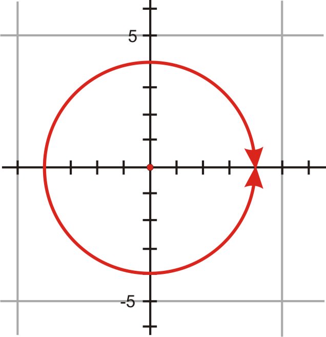
F-d_5822d9a38802a2b0f3969220b1b9367c7bbfe2208c478197999ecbc2+image_tiny+image_tiny.jpg — Figura\(\PageIndex{5}\)

F-d_297f46530cda774d3b1ccc84b43aa89df6689d1573838b3b338df990+image_tiny+image_tiny.jpg — Figura\(\PageIndex{5}\)

Ambas ecuaciones, una en forma rectangular y otra en forma polar, son círculos con un radio de 4 y centro en el origen.

2. Grafica las ecuaciones\((x−2)^2+(y+2)^2=8\) y\(r=4\cos \theta −4\sin \theta \). Describir las gráficas.

Aquí no se muestra una representación visual, pero en tu calculadora deberías ver que las gráficas son círculos centrados en\((2, -2)\) con un radio\(2\sqrt{2}\approx 2.8\).

Ejemplo\(\PageIndex{1}\)

Anteriormente, se le preguntó si hay alguna manera de determinar si las dos ecuaciones son equivalentes.

Solución

Como aprendiste en esta sección, podemos comparar gráficas de ecuaciones para ver si las ecuaciones son iguales o no.

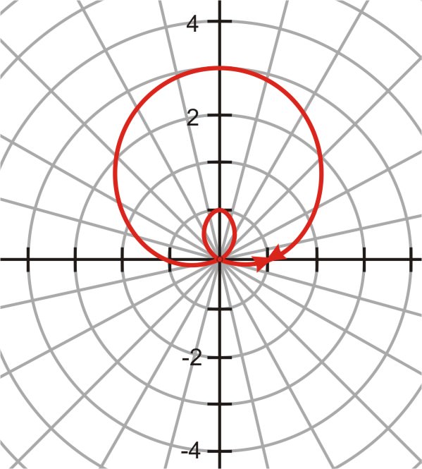
Un gráfico de\(3+2\cos (\theta )\) se ve así:

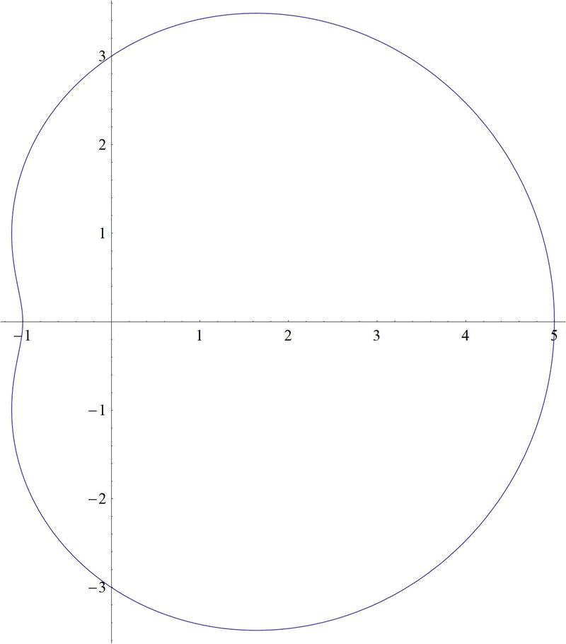
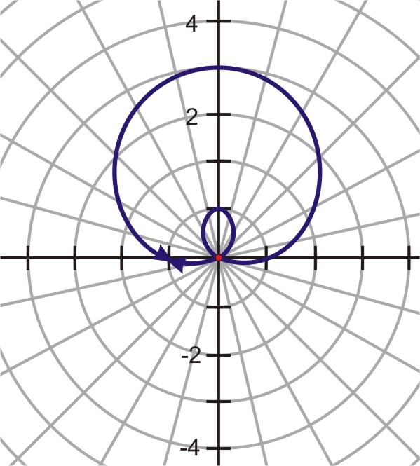
F-d_fce7965b9c263cd270a65e04d622375b732d278f8a637e070f6b12ad+image_tiny+image_tiny.jpg — Figura\(\PageIndex{6}\)

Y una gráfica de\(−3+2\cos (−\theta )\) se ve así:

Como puedes ver en las parcelas, tu amigo tiene razón. Tu gráfica y la suya son las mismas, por lo tanto las ecuaciones son equivalentes.

Ejemplo\(\PageIndex{2}\)

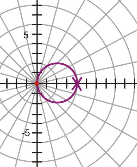
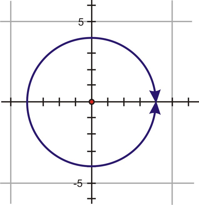
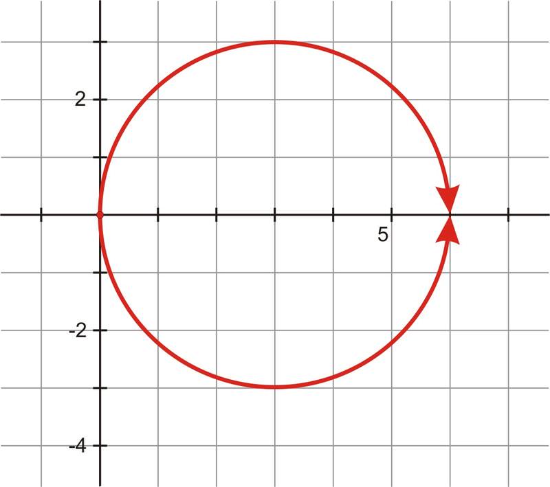
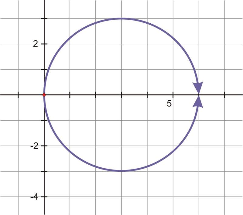
Escribe la ecuación rectangular\(x^2+y^2=6x\) en forma polar y grafica ambas ecuaciones. ¿Deberían ser equivalentes?

F-d_3af1fcdac2e39057e840359917e48fd346d5ace7b1b3618145243a3a3e+image_tiny+image_tiny.jpg — Figura\(\PageIndex{8}\)

f-d_a9b65cfd70867c11484e6d0868ab8fe7695c03072accbf6d15ade16c+image_tiny+image_tiny.jpg — Figura\(\PageIndex{9}\)

Solución

\ (\ begin {alineado}
x^ {2} +y^ {2} &=6 x & &\
r^ {2} &=6 (r\ cos\ theta) & & r^ {2} =x^ {2} +y^ {2}\ quad\ text {y}\ quad x=y\ cos\ theta\
r &=6\ cos\ theta &\ text dividir por} r
\ end {alineado}\)

Ambas ecuaciones produjeron un círculo con centro\((3,0)\) y un radio de 3.

Ejemplo\(\PageIndex{3}\)

Determinar si\(r=−2+\sin \theta \) y\(r=2−\sin \theta\) son equivalentes sin graficar.

Solución

\(r=−2+\sin \theta \)y no\(r=2−\sin \theta \) son equivalentes porque el seno tiene el signo contrario. \(r=−2+\sin \theta \)estará principalmente por encima del eje horizontal y\(r=2−\sin \theta \) estará mayormente por debajo. Sin embargo, los dos sí tienen las mismas intercepciones del eje polar.

Ejemplo\(\PageIndex{4}\)

Determinar si\(r=−3+4\cos (−\pi )\) y\(r=3+4\cos \pi\) son equivalentes sin graficar.

Solución

\(r=−3+4\cos (−\pi )\)y\(r=3+4\cos \pi \) son equivalentes porque el signo de “a” no importa, ni tampoco el signo de\(\theta \).

Revisar

Para cada ecuación en forma rectangular dada a continuación, escriba la ecuación equivalente en forma polar.

\(x^2+y^2=4\)
\(x^2+y^2=6y\)
\((x−1)^2+y^2=1\)
\((x−4)^2+(y−1)^2=17\)
\(x^2+y^2=9\)

Para cada ecuación a continuación en forma polar, escriba otra ecuación en forma polar que produzca la misma gráfica.

\(r=4+3\sin \theta\)
\(r=2−\sin \theta\)
\(r=2+2\cos \theta\)
\(r=3−\cos \theta\)
\(r=2+\sin \theta\)

Determinar si cada uno de los siguientes conjuntos de ecuaciones produce gráficas equivalentes sin graficar.

\(r=3−\sin \theta \)y\(r=3+\sin \theta\)
\(r=1+2\sin \theta \)y\(r=−1+2\sin \theta\)
\(r=3\sin \theta \)y\(r=3\sin (−\theta )\)
\(r=2\cos \theta \)y\(r=2\cos (−\theta )\)
\(r=1+3\cos \theta \)y\(r=1−3\cos \theta\)

Reseña (Respuestas)

Para ver las respuestas de Revisar, abra este archivo PDF y busque la sección 6.8.

Recursos adicionales

Práctica: Curvas polares equivalentes