
6.3: Líneas Terminadas
- Page ID
- 86595

Si, por otro lado, tenemos una línea finita terminada con alguna impedancia de carga, tenemos un problema algo más complicado de tratar, como se muestra en la Figura\(\PageIndex{1}\).
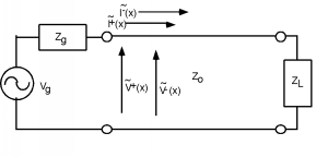
Figura\(\PageIndex{1}\): A Finite Terminated Transmission Line
There are several things we should note before we head off into equation-land again. First of all, unlike the transient problems we looked at in a previous chapter, there can be no more than two voltage and current signals on the line, just and , (and and ). We no longer have the luxury of having , , etc., because we are talking now about a steady state system. All of the transient solutions which built up when the generator was first connected to the line have been summed together into just two waves.
Thus, on the line we have a single total voltage function, which is just the sum of the positive and negative going voltage waves
and a total current function
Note also that until we have solved for and , we do not know or anywhere on the line. In particular, we do not know and which would tell us what the apparent impedance is looking into the line.
Until we know what kind of impedance the generator is seeing, we can not figure out how much of the generator's voltage will be coupled to the line! The input impedance looking into the line is now a function of the load impedance, the length of the line, and the phase velocity on the line. We have to solve this before we can figure out how the line and generator will interact.
The approach we shall have to take is the following. We will start at the load end of the line, and in a manner similar to the one we used previously, find a relationship between and , leaving their actual magnitude and phase as something to be determined later. We can then propagate the two voltages (and currents) back down to the input, determine what the input impedance is by finding the ratio of () to (), and from this, and knowledge of properties of the generator and its impedance, determine what the actual voltages and currents are.
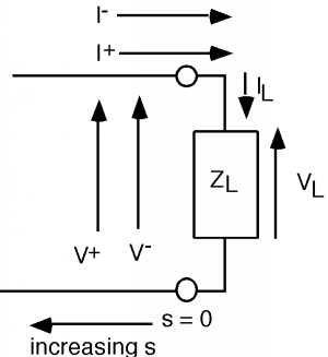
Let's take a look at the load. We again use KVL and KCL (Figure \(\PageIndex{2}\)) to match voltages and currents in the line and voltages and currents in the load:
and
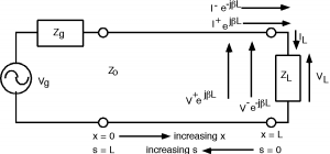
Ahora, podríamos sustituirpara las dos corrientes en la línea ypara, y luego tratar de resolver paraen términos deusando Ecuación y Ecuación, pero podemos ser un poco inteligentes al principio y hacer que nuestro álgebra (complejo) sea un poco más limpio, como se muestra en la Figura\(\PageIndex{3}\). Hagamos un cambio de variable y vamos
Figura\(\PageIndex{3}\): \(s=0\) at the load, and so the exponentials go away!
This then gives us for the voltage on the line (using )
Usually, we just fold the (constant) phase terms terms in with the and and so we have:
Note that when we do this, we now have a positive exponential in the first term associated with and a negative exponential associated with the term. Of course, we also get for :
This change now moves our origin to the load end of the line, and reverses the direction of positive motion. But, now when we plug into the value for at the load (), the equations simplify to:
and
which we then re-write as
This is beginning to look almost exactly like a previous chapter. As a reminder, we solve Equation for
and substitute for in Equation
From which we then solve for the reflection coefficient , the ratio of to .
Note that since, in general, will be complex, we can expect that will also be a complex number with both a magnitude and a phase angle . Also, as with the case when we were looking at transients, .
Since we now know in terms of , we can now write an expression for the voltage anywhere on the line.
Note again the change in signs in the two exponentials. Since our spatial variable is going in the opposite direction from , the phasor now goes as and the phasor now goes as .
We now substitute in for in Equation, and for reasons that will become apparent soon, factor out an .
We could have also written down an equation for , the current along the line. It will be a good test of your understanding of the basic equations we are developing here to show yourself that indeed