
5.7: Ejercicios
- Page ID
- 83373

A menos que se especifique lo contrario, use\(\beta\) = 100.
5.7.1: Problemas de análisis
1. Trazar la línea de carga para el circuito de la Figura\(\PageIndex{1}\). \(V_{CC}\)= 20 V,\(V_{EE}\) = −8 V,\(R_B\) = 7.5 k\(\Omega\),\(R_E\) = 10 k\(\Omega\),\(R_C\) = 12 k\(\Omega\).
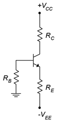
Figura\(\PageIndex{1}\)
2. Determine el nuevo punto Q para el Problema 1 si\(\beta\) = 250.
3. Trazar la línea de carga para el circuito de la Figura\(\PageIndex{2}\). \(V_{EE}\)= 5 V,\(V_{CC}\) = −18 V,\(R_B\) = 22 k\(\Omega\),\(R_E\) = 1.2 k\(\Omega\),\(R_C\) = 1.5 k\(\Omega\).
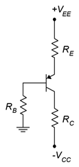
Figura\(\PageIndex{2}\)
4. Determine el nuevo punto Q para el Problema 3 si\(\beta\) = 50.
5. Trazar la línea de carga para el circuito de la Figura\(\PageIndex{3}\). \(V_{CC}\)= 20 V,\(R_1\) = 15 k\(\Omega\),\(R_2\) = 5 k\(\Omega\),\(R_E\) = 4.3 k\(\Omega\),\(R_C\) = 9.1 k\(\Omega\).
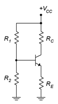
Figura\(\PageIndex{3}\)
6. Determine el nuevo punto Q para el Problema 5 si\(\beta\) = 150.
7. Trazar la línea de carga para el circuito de la Figura\(\PageIndex{4}\). \(V_{EE}\)= 16 V,\(R_1\) = 12 k\(\Omega\),\(R_2\) = 4.7 k\(\Omega\),\(R_E\) = 6.2 k\(\Omega\),\(R_C\) = 10 k\(\Omega\).
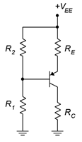
Figura\(\PageIndex{4}\)
8. Determine el nuevo punto Q para el Problema 7 si\(\beta\) = 200.
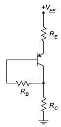
9. Trazar la línea de carga para el circuito de la Figura\(\PageIndex{5}\). \(V_{CC}\)= 12 V,\(R_B\) = 560 k\(\Omega\),\(R_C\) = 3.3 k\(\Omega\).
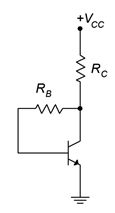
Figura\(\PageIndex{5}\)
10. Determine el nuevo punto Q para el Problema 9 si\(\beta\) = 75.
11. Trazar la línea de carga para el circuito de la Figura\(\PageIndex{6}\).
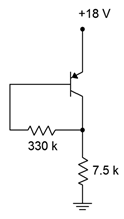
Figura\(\PageIndex{6}\)
12. Determine el nuevo punto Q para el Problema 11 si\(\beta\) = 200.
13. Trazar la línea de carga para el circuito de la Figura\(\PageIndex{7}\). \(V_{CC}\)= 15 V,\(R_B\) = 470 k\(\Omega\),\(R_E\) = 560\(\Omega\),\(R_C\) = 3.3 k\(\Omega\).
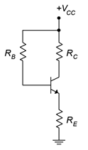
Figura\(\PageIndex{7}\)
14. Determine el nuevo punto Q para el Problema 13 si\(\beta\) = 170.
15. Trazar la línea de carga para el circuito de la Figura\(\PageIndex{8}\).
16. Determine el nuevo punto Q para Problema 15 si\(\beta\) = 75.
17. Trazar la línea de carga para el circuito de la Figura\(\PageIndex{9}\). \(V_{EE}\)= 18 V,\(R_B\) = 680 k\(\Omega\),\(R_E\) = 270\(\Omega\),\(R_C\) = 3.9 k\(\Omega\).
18. Determine el nuevo punto Q para el Problema 17 si\(\beta\) = 200.
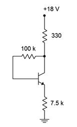
Figura\(\PageIndex{8}\)
Figura\(\PageIndex{9}\)
5.7.2: Problemas de diseño
19. Determinar un valor para\(R_E\) en el circuito de la Figura\(\PageIndex{1}\) para establecer\(I_C\) = 2 mA. Uso\(V_{CC}\) = 20 V,\(V_{EE}\) = −8 V,\(R_B\) = 10 k\(\Omega\),\(R_C\) = 5.6 k\(\Omega\).
20. Determinar un valor para\(R_C\) en el circuito de la Figura\(\PageIndex{2}\) para establecer\(V_{CE}\) = 10 V. Uso\(V_{CC}\) = −25 V,\(V_{EE}\) = 6 V,\(R_B\) = 15 k\(\Omega\),\(R_E\) = 6.8 k\(\Omega\).
21. Determinar un valor para\(R_C\) en el circuito de la Figura\(\PageIndex{3}\) para establecer\(V_{CE}\) = 8 V. Uso\(V_{CC}\) = 24 V,\(R_1\) = 22 k\(\Omega\),\(R_2\) = 10 k\(\Omega\),\(R_E\) = 5.6 k\(\Omega\).
22. Determinar nuevos valores para\(R_1\) y\(R_2\) en el circuito de la Figura\(\PageIndex{4}\) para establecer\(I_C\) = 500\(\mu\) A.\(V_{EE}\) = 22 V,\(R_E\) = 15 k\(\Omega\),\(R_C\) = 6.8 k\(\Omega\).
5.7.3: Problemas de desafío
23. Determine los valores máximo y mínimo para\(I_C\) en el Problema 1 si cada resistencia tiene una tolerancia del 10%.
24. Determine los valores máximo y mínimo para\(V_{CE}\) en el Problema 3 si cada resistencia tiene una tolerancia del 5%.
25. Determinar un valor para\(R_E\) en el circuito de la Figura\(\PageIndex{3}\) para establecer\(V_{CE}\) = 10 V.\(V_{CC}\) = 30 V,\(R_1\) = 12 k\(\Omega\),\(R_2\) = 3 k\(\Omega\),\(R_C\) = 8.2 k\(\Omega\).
26. Derivar Ecuación 5.16.
27. Determinar la potencia extraída de la fuente para el circuito de Problema 5. 28. Usando una fuente de alimentación de 15 voltios, diseñe un circuito de polarización para crear un punto Q muy estable de 2 mA y 5 voltios.
5.7.4: Problemas de simulación por computadora
29. Realizar una serie de simulaciones de CC para probar la estabilidad\(\beta\) del punto Q frente al circuito del Problema 1.
30. Realizar una simulación Monte Carlo para investigar la estabilidad del punto Q del circuito del Problema 5 si la resistencia del emisor tiene una tolerancia del 10%.