6.10: Ejercicios

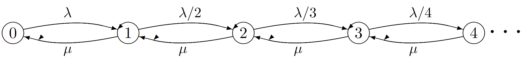
Ejercicio 6.1. Considere una cola M/M/1 como se representa en la Figura 6.4. Asumir a lo largo de ese\(X_0 = i\) donde\(i > 0\) El propósito de este ejercicio es comprender la relación entre el intervalo de retención hasta la siguiente transición de estado y el intervalo hasta la siguiente llegada a la cola M/M/1. Sus explicaciones en las siguientes partes pueden y deben ser muy breves.

a) Explique por qué es el intervalo de retención esperado\(\mathsf{E} [U_1|X_0 = i]\) hasta la siguiente transición de estado\(1/(\lambda+\mu)\).

b) Explicar por qué el intervalo de retención esperado\(U_1\), condicional\(X_0 = i\) y\(X_1 = i + 1\), es

\[\mathsf{E}[U_1|X_0=i, X_1=i+1]=1/(\lambda+\mu) \nonumber \]

Demostrar que\(\mathsf{E}[U_1|X_0=i,X_1=i-1]\) es lo mismo

c)\(V\) Sea la hora de la primera llegada después del tiempo 0 (esto puede ocurrir ya sea antes o después de la hora\(W\) de la primera salida.) Demostrar que

\[\begin{aligned} \mathsf{E}[V|X_0=i, X_1=i+1] \quad &=\quad \dfrac{1}{\lambda+\mu} \\ \mathsf{E}[V|X_0=i, X_1=i-1] \quad &= \quad \dfrac{1}{\lambda+\mu} + \dfrac{1}{\lambda} \end{aligned} \nonumber \]

Pista: En la segunda ecuación, use la falta de memoria del rv exponencial y el hecho de que V bajo esta condición es el tiempo hasta la primera salida más el tiempo restante para una llegada.

d) Usa tu solución para la parte c) más la probabilidad de subir o bajar en la cadena de Markov para demostrarlo\(\mathsf{E} [V ] = 1/\lambda\). (Nota: ya lo sabes\(\mathsf{E} [V ] = 1 /\lambda\). El propósito aquí es demostrar que su solución a la parte c) es consistente con ese hecho.)

Ejercicio 6.2. Consideremos un proceso de Markov para el cual la cadena incrustada de Markov es una cadena de nacer-muerte con probabilidades de transición\(P_{i,i+1} = 2/5\) para todos\(i \geq 0, P_{i,i-1} = 3/5\) para todos\(i \geq 1\)\(P_{01} = 1\), y de\(P_{ij} = 0\) otra manera.

a) Encontrar las probabilidades de estado estacionario\(\{\pi_i; i \geq 0\}\) para la cadena incrustada.

b) Supongamos que la tasa de transición\(\nu_i\) fuera del estado\(i\), para\(i \geq 0\), viene dada por\(\nu_i = 2^i\). Encontrar las tasas de transición\(\{ q_{ij} \}\) entre estados y encontrar las probabilidades de estado estacionario\(\{p_i\}\) para el proceso de Markov. Explique heurísticamente por qué\(\pi_i \neq p_i\).

c) Explicar por qué no existe una aproximación de tiempo muestreado para este proceso. Luego trunca la cadena incrustada a estados 0\(m\) y encuentra las probabilidades de estado estacionario para la aproximación de tiempo muestreado al proceso truncado.

d) Demostrar que como\(m \rightarrow \infty\), las probabilidades de estado estacionario para la secuencia de aproximaciones de tiempo muestreado se aproximan a las probabilidades\(p_i\) en la parte b).

Ejercicio 6.3. Consideremos un proceso de Markov para el cual la cadena incrustada de Markov es una cadena de nacer-muerte con probabilidades de transición\(P_{i,i+1} = 2/5\) para todos\(i \geq 1\),\(P_{i,i-1} = 3/5\) para todos\(i \geq 1\)\(P_{01} = 1\), y de\(P_{ij} = 0\) otra manera.

a) Encontrar las probabilidades de estado estacionario\(\{\pi_i; i \geq 0\}\) para la cadena incrustada.

b) Supongamos que la tasa de transición fuera del estado\(i\), para\(i \geq 0\), viene dada por\(\nu_i = 2^{-i}\). Encuentre las tasas de transición\(\{q_{ij} \}\) entre estados y muestre que no existe una solución de vector de probabilidad\(\{p_i; i \geq 0\}\) a (6.2.17).

c) Argumentan que el tiempo esperado entre visitas a cualquier estado dado\(i\) es infinito. Encuentra el número esperado de transiciones entre visitas a cualquier estado dado\(i\). Argumentan que, a partir de cualquier estado\(i\),\(i\) se produce un eventual retorno al estado con probabilidad 1.

d) Considerar la aproximación de tiempo muestreado de este proceso con\(\delta = 1\). Dibuja la gráfica de la cadena resultante de Markov y argumenta por qué debe ser nula recurrente.

Ejercicio 6.4. Considere el proceso de Markov para la cola M/M/1, como se indica en la Figura 6.4.

a) Encontrar las probabilidades de proceso en estado estacionario (en función de\(\rho = \lambda/\mu)\) desde (6.2.9) y también como la solución a (6.2.17). Verificar que las dos soluciones sean iguales.

b) Para las partes restantes del ejercicio, supongamos que\(\rho = 0.01\), asegurando así (para ayudar a la intuición) que los estados 0 y 1 son mucho más probables que los demás estados. Supongamos que el proceso ha estado funcionando desde hace mucho tiempo y se encuentra en estado estacionario. Explica con tus propias palabras la diferencia entre\(\pi_1\) (la probabilidad de estado estacionario del estado 1 en la cadena incrustada) y\(p_1\) (la probabilidad de estado estacionario de que el proceso esté en estado 1. De manera más explícita, qué experimentos podrías realizar (repetidamente) sobre el proceso a medir\(\pi_1\) y\(p_1\).

c) Ahora suponga que desea iniciar el proceso en estado estacionario. Demostrar que es imposible elegir probabilidades iniciales para que tanto el proceso como la cadena incrustada comiencen en estado estacionario. ¿Qué versión de estado estacionario es la más cercana a su vista intuitiva? (Aquí no hay una respuesta correcta, pero es importante darse cuenta de que la noción de estado estacionario no es tan simple como se podría imaginar).

d) Dejar\(M (t)\) ser el número de transiciones (contando tanto llegadas como salidas) que tienen lugar por tiempo\(t\) en este proceso de Markov y asumir que la cadena incrustada de Markov inicia en estado estacionario en el tiempo 0. Let\(U_1, U_2, . . . \), ser la secuencia de intervalos de retención entre transiciones (\(U_1\)siendo el tiempo a la primera transición). Demuestre que estos rv están distribuidos de manera idéntica. Mostrar con el ejemplo que no son independientes (\(i.e.\), no\(M (t)\) es un proceso de renovación).

Ejercicio 6.5. Considera el proceso de Markov que se ilustra a continuación. Las transiciones están etiquetadas por la velocidad\(q_{ij}\) a la que ocurren esas transiciones. El proceso se puede ver como una cola de servidor único donde las llegadas se desaniman cada vez más a medida que la cola se alarga. La palabra promedio de tiempo a continuación se refiere al promedio de tiempo limitante sobre cada ruta de muestra del proceso, excepto para un conjunto de rutas de muestra de probabilidad 0.

a) Encontrar la fracción de tiempo promedio\(p_i\) spent in each state \(i > 0\) in terms of \(p_0\) and then solve for \(p_0\). Hint: First find an equation relating \(p_i\) to \(p_{i+1}\) for each \(i\). It also may help to recall the power series expansion of \(e^x\).

b) Find a closed form solution to \(\sum_i p_i\nu_i\) where \(\nu_i\) is the departure rate from state \(i\). Show that the process is positive recurrent for all choices of \(\lambda >0\) and \(\mu>0\) and explain intuitively why this must be so.

c) For the embedded Markov chain corresponding to this process, find the steady-state probabilities \(\pi_i\) for each \(i \geq 0\) and the transition probabilities \(P_{ij}\) for each \(i, j\).

d) For each \(i\), find both the time-average interval and the time-average number of overall state transitions between successive visits to \(i\).

Exercise 6.6. (Detail from proof of Theorem 6.2.1)

a) Let \(U_n\) be the \(n\)th holding interval for a Markov process starting in steady state, with \(\text{Pr}\{X_0 = i\} = \pi_i\). Show that \(\mathsf{E} [U_n] =\sum_k \pi_k/\nu_k\) for each integer \(n\).

b) Let \(S_n\) be the epoch of the \(n\)th transition. Show that \(\text{Pr}\{ S_n \geq n\beta \}\leq \frac{\sum_k \pi_k/\nu_k}{\beta}\) for all \(\beta > 0\).

c) Let \(M (t)\) be the number of transitions of the Markov process up to time \(t\), given that \(X_0\) is in steady state. Show that \(\text{Pr}\{ M (n \beta) < n\} >1-\frac{\sum_k \pi_k\nu_k}{\beta} \).

d) Show that if \(\sum_k \pi_k/\nu_k\) is finite, then \(\lim_{t\rightarrow \infty} M (t)/t = 0\) WP1 is impossible. (Note that this is equivalent to showing that \(\lim_{t\rightarrow \infty} M (t)/t = 0\) WP1 implies \(\sum_k \pi_k/\nu_k = \infty\)).

e) Let \(M_i(t)\) be the number of transitions by time \(t\) starting in state \(i\). Show that if \(\sum_k \pi_k/\nu_k\) is finite, then \(\lim_{t\rightarrow \infty} M_i(t)/t = 0\) WP1 is impossible.

Exercise 6.7.

a) Consider the process in the figure below. The process starts at \(X(0) = 1\), and for all \(i \geq 1\), \(P_{i,i+1} = 1\) and \(\nu_i = i^2\) for all \(i\). Let \(S_n\) be the epoch when the \(n^{th}\) transition occurs. Show that

\[\mathsf{E} [S_n] = \sum^n_{i=1} i^{-2} <2 \text{ for all } n\nonumber \]

Hint: Upper bound the sum from \(i = 2\) by integrating \(x^{-2}\) from \(x=1\).

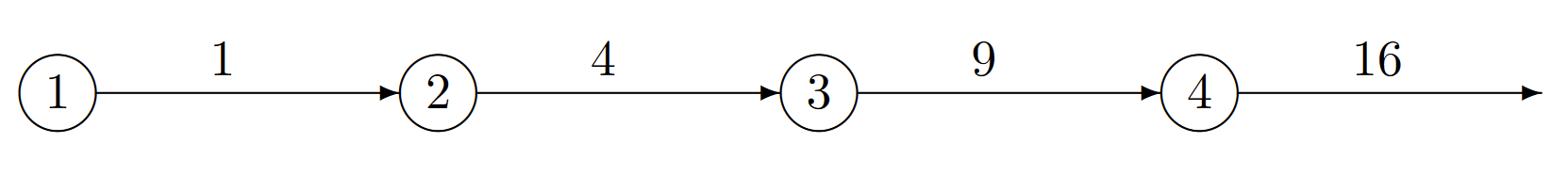
b) Use the Markov inequality to show that \(\text{Pr}\{ S_n > 4\} \leq 1/2\) for all \(n\). Show that the probability of an infinite number of transitions by time 4 is at least 1/2.

Exercise 6.8.

a) Consider a Markov process with the set of states \(\{0, 1, . . . \}\) in which the transition rates \(\{ q_{ij}\}\) between states are given by \(q_{i,i+1} = (3/5)2^i\) for \(i \geq 0\), \(q_{i,i-1} = \ref{2/5} 2^i\) for \(i\geq 1\), and \(q_{ij} = 0\) otherwise. Find the transition rate \(\nu_i\) out of state \(i\) for each \(i \geq 0\) and find the transition probabilities \(\{ P_{ij} \}\) for the embedded Markov chain.

b) Find a solution \(\{ p_i; i \geq 0\}\) with \(\sum_i p_i = 1\) to (6.2.17).

c) Show that all states of the embedded Markov chain are transient.

d) Explain in your own words why your solution to part b) is not in any sense a set of steady-state probabilities

Exercise 6.9. Let \(q_{i,i+1} = 2^{i-1}\) for all \(i \geq 0\) and let \(q_{i,i-1} = 2^{i-1}\) for all \(i\geq 1\). All other transition rates are 0.

a) Solve the steady-state equations and show that \(p_i = 2^{-i-1}\) for all \(i\geq 0\).

b) Find the transition probabilities for the embedded Markov chain and show that the chain is null recurrent.

c) For any state \(i\), consider the renewal process for which the Markov process starts in state \(i\) and renewals occur on each transition to state \(i\). Show that, for each \(i \geq 1\), the expected inter-renewal interval is equal to 2. Hint: Use renewal-reward theory.

d) Show that the expected number of transitions between each entry into state \(i\) is infinite. Explain why this does not mean that an infinite number of transitions can occur in a finite time.

Exercise 6.10.

a) Consider the two state Markov process of Example 6.3.1 with \(q_{01} = \lambda\) and \(q_{10} = μ\). Find the eigenvalues and eigenvectors of the transition rate matrix \([Q]\).

b) If \([Q]\) has \(\mathsf{M}\) distinct eigenvalues, the differential equation \(d[P (t)]/dt = [Q][P (t)]\) can be solved by the equation

\[ [P(t)] = \sum^{\mathsf{M}}_{i=1} \boldsymbol{\nu}_i e^{t\lambda_i}\boldsymbol{p}^{\mathsf{T}}_i \nonumber \]

where \(\boldsymbol{p}_i\) and \(\boldsymbol{\nu}_i\) are the left and right eigenvectors of eigenvalue \(\lambda_i\). Show that this equation gives the same solution as that given for Example 6.3.1.

Exercise 6.11. Consider the three state Markov process below; the number given on edge \((i, j)\) is \(q_{ij}\), the transition rate from \(i\) to \(j\). Assume that the process is in steady state.

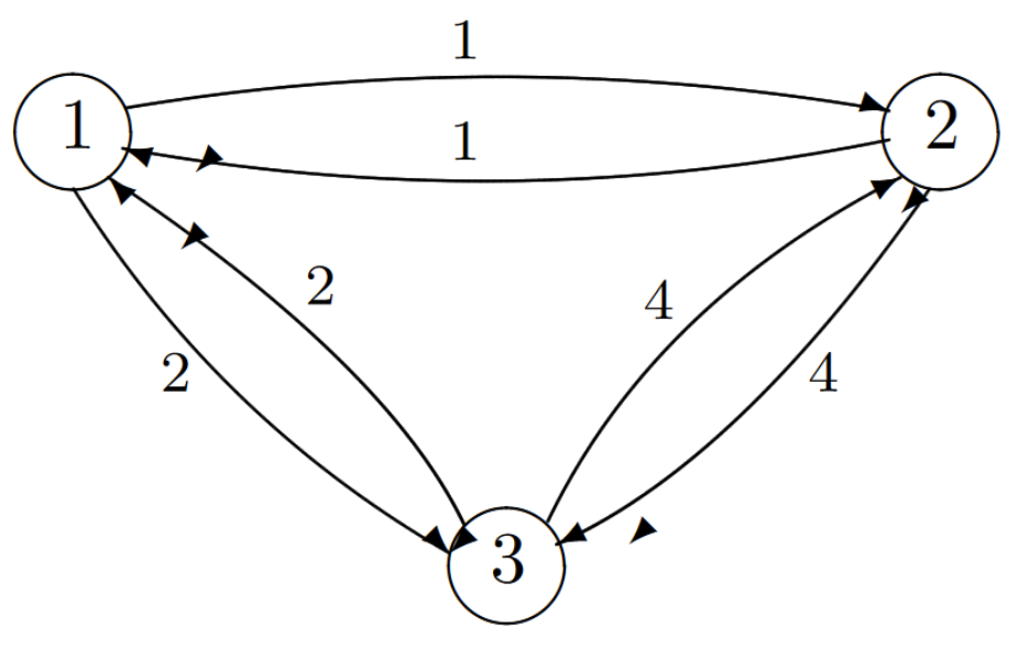
a) Is this process reversible?

b) Find \(p_i\), the time-average fraction of time spent in state \(i\) for each \(i\).

c) Given that the process is in state \(i\) at time \(t\), find the mean delay from \(t\) until the process leaves state \(i\).

d) Find \(\pi_i\), the time-average fraction of all transitions that go into state \(i\) for each \(i\).

e) Suppose the process is in steady state at time \(t\). Find the steady state probability that the next state to be entered is state 1.

f) Given that the process is in state 1 at time \(t\), find the mean delay until the process first returns to state 1.

g) Consider an arbitrary irreducible finite-state Markov process in which \(q_{ij} = q_{ji}\) for all \(i, j\). Either show that such a process is reversible or find a counter example.

Exercise 6.12.

a) Consider an M/M/1 queueing system with arrival rate \(\lambda \), service rate \(\mu\), \(\mu>\lambda\). Assume that the queue is in steady state. Given that an arrival occurs at time \(t\), find the probability that the system is in state \(i\) immediately after time \(t\).

b) Assuming FCFS service, and conditional on \(i\) customers in the system immediately after the above arrival, characterize the time until the above customer departs as a sum of random variables.

c) Find the unconditional probability density of the time until the above customer de­parts.

Hint: You know (from splitting a Poisson process) that the sum of a geometrically distributed number of IID exponentially distributed random variables is exponentially dis­tributed. Use the same idea here.

Exercise 6.13.

a) Consider an M/M/1 queue in steady state. Assume \( \rho = \lambda / \mu <1\). Find
the probability \(Q(i, j)\) for \(i \geq j>0\) that the system is in state \(i\) at time \(t\) and that \(i -j\) departures occur before the next arrival.

b) Find the PMF of the state immediately before the first arrival after time \(t\).

c) There is a well-known queueing principle called PASTA, standing for “Poisson arrivals see time-averages”. Given your results above, give a more precise statement of what that principle means in the case of the M/M/1 queue.

Exercise 6.14. A small bookie shop has room for at most two customers. Potential cus­tomers arrive at a Poisson rate of 10 customers per hour; they enter if there is room and are turned away, never to return, otherwise. The bookie serves the admitted customers in order, requiring an exponentially distributed time of mean 4 minutes per customer.

a) Find the steady-state distribution of number of customers in the shop.

b) Find the rate at which potential customers are turned away.

c) Suppose the bookie hires an assistant; the bookie and assistant, working together, now serve each customer in an exponentially distributed time of mean 2 minutes, but there is only room for one customer (\(i.e.\), the customer being served) in the shop. Find the new rate at which customers are turned away.

Exercise 6.15. This exercise explores a continuous time version of a simple branching process.

Consider a population of primitive organisms which do nothing but procreate and die. In particular, the population starts at time 0 with one organism. This organism has an exponentially distributed lifespan \(T_0\) with rate \(μ\) (\(i.e.\), \(\text{Pr}\{T_0 \geq \tau\} = e^{-\mu\tau} \)). While this organism is alive, it gives birth to new organisms according to a Poisson process of rate \(\lambda\). Each of these new organisms, while alive, gives birth to yet other organisms. The lifespan and birthrate for each of these new organisms are independently and identically distributed to those of the first organism. All these and subsequent organisms give birth and die in the same way, again independently of all other organisms.

a) Let \(X(t)\) be the number of (live) organisms in the population at time \(t\). Show that \(\{ X(t); t \geq 0\}\) is a Markov process and specify the transition rates between the states.

b) Find the embedded Markov chain \(\{ X_n; n \geq 0\}\) corresponding to the Markov process in part a). Find the transition probabilities for this Markov chain.

c) Explain why the Markov process and Markov chain above are not irreducible. Note: The majority of results you have seen for Markov processes assume the process is irreducible, so be careful not to use those results in this exercise.

d) For purposes of analysis, add an additional transition of rate \(\lambda\) from state 0 to state 1. Show that the Markov process and the embedded chain are irreducible. Find the values of \(\lambda\) and \(μ\) for which the modified chain is positive recurrent, null-recurrent, and transient.

e) Assume that \(\lambda < μ\). Find the steady state process probabilities for the modified Markov process.

f) Find the mean recurrence time between visits to state 0 for the modified Markov process.

g) Find the mean time \(\overline{T}\) for the population in the original Markov process to die out. Note: We have seen before that removing transitions from a Markov chain or process to create a trapping state can make it easier to find mean recurrence times. This is an example of the opposite, where adding an exit from a trapping state makes it easy to find the recurrence time.

Exercise 6.16. Consider the job sharing computer system illustrated below. Incoming jobs arrive from the left in a Poisson stream. Each job, independently of other jobs, requires pre-processing in system 1 with probability \(Q\). Jobs in system 1 are served FCFS and the service times for successive jobs entering system 1 are IID with an exponential distribution of mean \(1/μ_1\). The jobs entering system 2 are also served FCFS and successive service times are IID with an exponential distribution of mean \(1/μ_2\). The service times in the two systems are independent of each other and of the arrival times. Assume that \(μ_1 > \lambda Q\) and that \(μ_2 > \lambda\). Assume that the combined system is in steady state.

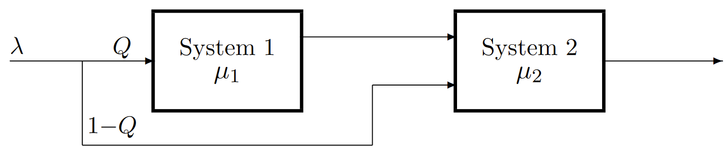
a) Is the input to system 1 Poisson? Explain.

b) Are each of the two input processes coming into system 2 Poisson? Explain.

c) Give the joint steady-state PMF of the number of jobs in the two systems. Explain briefly.

d) What is the probability that the first job to leave system 1 after time \(t\) is the same as the first job that entered the entire system after time \(t\)?

e) What is the probability that the first job to leave system 2 after time \(t\) both passed through system 1 and arrived at system 1 after time \(t\)?

Exercise 6.17. Consider the following combined queueing system. The first queue system is M/M/1 with service rate \(μ_1\). The second queue system has IID exponentially distributed service times with rate \(μ_2\). Each departure from system 1 independently \(1 - Q_1\). System 2 has an additional Poisson input of rate \(\lambda_2\), independent of inputs and outputs from the first system. Each departure from the second system independently leaves the combined system with probability \(Q_2\) and re-enters system 2 with probability \(1 -Q_2\). For parts a), b), c) assume that \(Q2 = 1\) (\(i.e.\), there is no feedback).

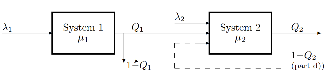
a) Characterize the process of departures from system 1 that enter system 2 and characterize the overall process of arrivals to system 2.

b) Assuming FCFS service in each system, find the steady state distribution of time that a customer spends in each system.

c) For a customer that goes through both systems, show why the time in each system is independent of that in the other; find the distribution of the combined system time for such a customer.

d) Now assume that \(Q_2 < 1\). Is the departure process from the combined system Poisson? Which of the three input processes to system 2 are Poisson? Which of the input processes are independent? Explain your reasoning, but do not attempt formal proofs.

Exercise 6.18. Suppose a Markov chain with transition probabilities \(\{ P_{ij} \}\) is reversible. Suppose we change the transition probabilities out of state 0 from \(\{ P_{0j} ; j \geq 0\}\) to \(\{ P_{0j}'; j\geq 0\}\). Assuming that all \(P_{ij}\) for \(i \neq 0\) are unchanged, what is the most general way in which we can choose \(\{ P_{0j}' ; j \geq 0\}\) so as to maintain reversibility? Your answer should be explicit0j about how the steady-state probabilities \(\{ \pi_i; i \geq 0\}\) are changed. Your answer should also indicate what this problem has to do with uniformization of reversible Markov processes, if anything.

Hint: Given \(P_{ij}\) for all \(i, j\), a single additional parameter will suffice to specify \(P_{0j}'\) for all \(j\).

Exercise 6.19. Consider the closed queueing network in the figure below. There are three customers who are doomed forever to cycle between node 1 and node 2. Both nodes use FCFS service and have exponentially distributed IID service times. The service times at one node are also independent of those at the other node and are independent of the customer being served. The server at node \(i\) has mean service time \(1/μ_i\), \(i = 1, 2\). Assume to be specific that \(μ_2 < μ_1\).

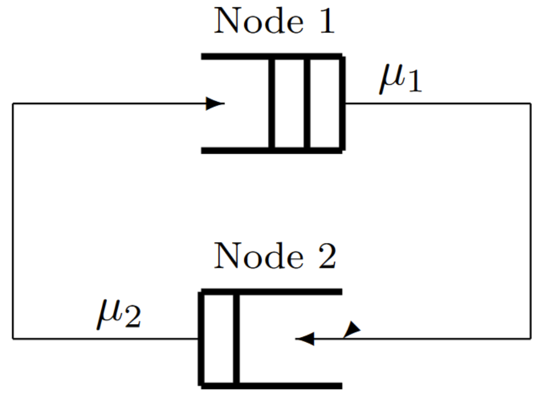
a) The system can be represented by a four state Markov process. Draw its graphical representation and label it with the individual states and the transition rates between them.

b) Find the steady-state probability of each state.

c) Find the time-average rate at which customers leave node 1.

d) Find the time-average rate at which a given customer cycles through the system.

e) Is the Markov process reversible? Suppose that the backward Markov process is inter­preted as a closed queueing network. What does a departure from node 1 in the forward process correspond to in the backward process? Can the transitions of a single customer in the forward process be associated with transitions of a single customer in the backward process?

Exercise 6.20. Consider an M/G/1 queueing system with last come first serve (LCFS) pre-emptive resume service. That is, customers arrive according to a Poisson process of rate \(\lambda\). A newly arriving customer interrupts the customer in service and enters service itself. When a customer is finished, it leaves the system and the customer that had been interrupted by the departing customer resumes service from where it had left off. For example, if customer 1 arrives at time 0 and requires 2 units of service, and customer 2 arrives at time 1 and requires 1 unit of service, then customer 1 is served from time 0 to 1; customer 2 is served from time 1 to 2 and leaves the system, and then customer 1 completes service from time 2 to 3. Let \(X_i\) be the service time required by the \(i^{th}\) customer; the \(X_i\) are IID random variables with expected value \(\mathsf{E} [X]\); they are independent of customer arrival times. Assume \(\lambda \mathsf{E}[X]<1\).

a) Find the mean time between busy periods (\(i.e.\), the time until a new arrival occurs after the system becomes empty).

b) Find the time-average fraction of time that the system is busy.

c) Find the mean duration, \(\mathsf{E} [B]\), of a busy period. Hint: use a) and b).

d) Explain briefly why the customer that starts a busy period remains in the system for the entire busy period; use this to find the expected system time of a customer given that that customer arrives when the system is empty.

e) Is there any statistical dependence between the system time of a given customer (\(i.e.\), the time from the customer’s arrival until departure) and the number of customers in the system when the given customer arrives?

f) Show that a customer’s expected system time is equal to \(\mathsf{E} [B]\). Hint: Look carefully at your answers to d) and e).

g) Let \(C\) be the expected system time of a customer conditional on the service time \(X\) of that customer being 1. Find (in terms of \(C\)) the expected system time of a customer conditional on \(X = 2\); (Hint: compare a customer with \(X = 2\) to two customers with \(X = 1\) each); repeat for arbitrary \(X = x\).

h) Find the constant \(C\). Hint: use f) and g); don’t do any tedious calculations.

Exercise 6.21. Consider a queueing system with two classes of customers, type \(A\) and type \(B\). Type \(A\) customers arrive according to a Poisson process of rate \(\lambda_A\) and customers of type \(B\) arrive according to an independent Poisson process of rate \(\lambda_B\). The queue has a FCFS server with exponentially distributed IID service times of rate \(μ > \lambda_A + \lambda_B\). Characterize the departure process of class \(A\) customers; explain carefully. Hint: Consider the combined arrival process and be judicious about how to select between \(A\) and \(B\) types of customers.

Exercise 6.22. Consider a pre-emptive resume last come first serve (LCFS) queueing sys­tem with two classes of customers. Type \(A\) customer arrivals are Poisson with rate \(\lambda_A\) and Type \(B\) customer arrivals are Poisson with rate \(\lambda_B\). The service time for type \(A\) customers is exponential with rate \(μ_A\) and that for type \(B\) is exponential with rate \(μ_B\). Each service time is independent of all other service times and of all arrival epochs.

Define the “state” of the system at time \(t\) by the string of customer types in the system at \(t\), in order of arrival. Thus state \(AB\) means that the system contains two customers, one of type \(A\) and the other of type \(B\); the type \(B\) customer arrived later, so is in service. The set of possible states arising from transitions out of \(AB\) is as follows:

\(ABA\) if another type \(A\) arrives.

\(ABB\) if another type \(B\) arrives.

\(A\) if the customer in service (\(B\)) departs.

Note that whenever a customer completes service, the next most recently arrived resumes service, so the state changes by eliminating the final element in the string.

a) Draw a graph for the states of the process, showing all states with 2 or fewer customers and a couple of states with 3 customers (label the empty state as \(E\)). Draw an arrow, labelled by the rate, for each state transition. Explain why these are states in a Markov process.

b) Is this process reversible. Explain. Assume positive recurrence. Hint: If there is a transition from one state \(S\) to another state \(S'\), how is the number of transitions from \(S\) to \(S'\) related to the number from \(S'\) to \(S\)?

c) Characterize the process of type \(A\) departures from the system (\(i.e.\), are they Poisson?; do they form a renewal process?; at what rate do they depart?; etc.)

d) Express the steady-state probability \(\text{Pr}\{ A\}\) of state \(A\) in terms of the probability of the empty state \(\text{Pr}\{ E\}\). Find the probability \(\text{Pr}\{ AB\}\) and the probability \(\text{Pr}\{ ABBA\}\) in terms of \(\text{Pr}\{ E\}\). Use the notation \(\rho_A = \lambda_A/\mu_A\) and \(\rho_B=\lambda_B/\mu_B\).

e) Let \(Q_n\) be the probability of \(n\) customers in the system, as a function of \(Q_0 = \text{Pr}\{ E\}\). Show that \(Q_n = (1 -\rho ) \rho^n\) where \(\rho = \rho_A+\rho_B\).

Exercise 6.23.

a) Generalize Exercise 6.22 to the case in which there are \(m\) types of customers, each with independent Poisson arrivals and each with independent exponential service times. Let \(\lambda_i\) and \(\mu_i\) be the arrival rate and service rate respectively of the \(i^{th}\) user. Let \(\rho_i = \lambda_i / \mu_i\) and assume that \(\rho = \rho_1 + \rho_2 + ...+ \rho_m < 1\). In particular, show, as before that the probability of \(n\) customers in the system is \(Q_n = (1 -\rho ) \rho^n\) for \(0 \leq n<\infty\).

b) View the customers in part a) as a single type of customer with Poisson arrivals of rate \(\lambda = \sum_i \lambda_i\) and with a service density \(\sum_i (\lambda_i/\lambda) \mu_i \exp (-\mu_i x)\). Show that the expected service time is \(\rho/\lambda\). Note that you have shown that, if a service distribution can be represented as a weighted sum of exponentials, then the distribution of customers in the system for LCFS service is the same as for the M/M/1 queue with equal mean service time.

Exercise 6.24. Consider a \(k\) node Jackson type network with the modification that each node \(i\) has \(s\) servers rather than one server. Each server at \(i\) has an exponentially distributed service time with rate \(μ_i\). The exogenous input rate to node \(i\) is \(\rho_i = \lambda_0 Q_{0i}\) and each output from \(i\) is switched to \(j\) with probability \(Q_{ij}\) and switched out of the system with probability \(Q_{i0}\) (as in the text). Let \(\lambda_i, 1\leq i \leq k\), be the solution, for given \(\lambda_0\), to

\[ \lambda_j = \sum^k_{i=0} \lambda_i Q_{ij} \nonumber \]

\(1\leq j\leq k\) and assume that \(\lambda_i < s\mu_i\); \(1\leq i\leq k\). Show that the steady-state probability of state \(\boldsymbol{m}\) is

\[ \text{Pr} \{\boldsymbol{m}\} = \prod^k_{i=1} p_i (m_i) \nonumber \]

where \(p_i (m_i)\) is the probability of state \(m_i\) in an (M, M, s) queue. Hint: simply extend the argument in the text to the multiple server case.

Exercise 6.25. Suppose a Markov process with the set of states \(A\) is reversible and has steady-state probabilities \(p_i\); \(i \in A\). Let \(B\) be a subset of \(A\) and assume that the process is changed by setting \(q_{ij} = 0\) for all \(i\in B\), \(j \notin B\). Assuming that the new process (starting in \(B\) and remaining in \(B\)) is irreducible, show that the new process is reversible and find its steady-state probabilities.

Exercise 6.26. Consider a queueing system with two classes of customers. Type \(A\) cus­tomer arrivals are Poisson with rate \(\lambda_A\) and Type \(B\) customer arrivals are Poisson with rate \(\lambda_B\). The service time for type \(A\) customers is exponential with rate \(μ_A\) and that for type \(B\) is exponential with rate \(μ_B\). Each service time is independent of all other service times and of all arrival epochs.

a) First assume there are infinitely many identical servers, and each new arrival immediately enters an idle server and begins service. Let the state of the system be \((i, j)\) where \(i\) and \(j\) are the numbers of type \(A\) and \(B\) customers respectively in service. Draw a graph of the state transitions for \(i \leq 2\), \(j \leq 2\). Find the steady-state PMF, \(\{ p(i, j); i, j \geq 0\}\), for the Markov process. Hint: Note that the type \(A\) and type \(B\) customers do not interact.

b) Assume for the rest of the exercise that there is some finite number m of servers. Cus­tomers who arrive when all servers are occupied are turned away. Find the steady-state PMF, \(\{ p(i, j); i, j \geq 0, i+j \leq m\}\), in terms of \(p(0, 0)\) for this Markov process. Hint: Combine part a) with the result of Exercise 6.25.

c) Let \(Q_n\) be the probability that there are n customers in service at some given time in steady state. Show that \(Q_n = p(0, 0)\rho_n/n!\) for \(0 \leq n \leq m\) where \(\rho = \rho_A + \rho_B \), \(\rho_A = \lambda_A / \mu_A\) and \(\rho_B = \lambda_B / \mu_B\). Solve for \(p(0,0)\).

Exercise 6.27.

a) Generalize Exercise 6.26 to the case in which there are \(K\) types of customers, each with independent Poisson arrivals and each with independent exponential service times. Let \(\lambda_k\) and \(\mu_k\) be the arrival rate and service rate respectively for the \(k^h\) user type, \(1 \leq k \leq K\). Let \(\rho_k = \lambda_k/\mu_k\) and \(\rho = \rho_1 + \rho_2 + ...+ \rho_K\). In particular, show, as before, that the probability of \(n\) customers in the system is \(Q_n = p(0, . . . , 0)\rho_n/n!\) for \(0 \leq n \leq m\).

b) View the customers in part a) as a single type of customer with Poisson arrivals of rate \(\lambda = \sum_k \lambda_k\) and with a service density \(\sum_k (\lambda_k/\lambda ) \mu_k \exp -\mu_k x)\). Show that the expected service time is \(\rho/\lambda\). Note that what you have shown is that, if a service distribution can be represented as a weighted sum of exponentials, then the distribution of customers in the system is the same as for the M/M/m,m queue with equal mean service time.

Exercise 6.28. Consider a sampled-time M/D/m/m queueing system. The arrival process is Bernoulli with probability \(\lambda <<1 \) of arrival in each time unit. There are \(m\) servers; each arrival enters a server if a server is not busy and otherwise the arrival is discarded. If an arrival enters a server, it keeps the server busy for \(d\) units of time and then departs; \(d\) is some integer constant and is the same for each server.

Let \(n\), \(0 \leq n \leq m\) be the number of customers in service at a given time and let \(x_i\) be the number of time units that the \(i^{th}\) of those \(n\) customers (in order of arrival) has been in service. Thus the state of the system can be taken as \((n, \boldsymbol{x} ) = (n, x_1, x_2, . . . , x_n)\) where \(0 \leq n \leq m\) and \(1 \leq x_1 < x_2 < . . . < x_n \leq d\).

Let \(A(n, \boldsymbol{x} )\) denote the next state if the present state is \((n, \boldsymbol{x} )\) and a new arrival entersservice. That is,

\[ \begin{align} A(n,\boldsymbol{X}) \quad &= \quad (n+1,1,x_1+1,x_2+1,...,x_n+1) \quad \text{for } n<m \text{ and } x_n<d \\ A(n,\boldsymbol{X}) \quad &= \quad (n,1,x_1+1,x_2+1,...,x_{n-1} +1) \quad \text{for } n\leq m \text{ and } x_n=d \end{align} \nonumber \]

That is, the new customer receives one unit of service by the next state time, and all the old customers receive one additional unit of service. If the oldest customer has received \(d\) units of service, then it leaves the system by the next state time. Note that it is possible for a customer with \(d\) units of service at the present time to leave the system and be replaced by an arrival at the present time (\(i.e.\), (6.10.2) with \(n = m\), \(x_n = d\)). Let \(B(n, \boldsymbol{x} )\) denote the next state if either no arrival occurs or if a new arrival is discarded.

\[ \begin{align} B(n, \boldsymbol{x}) \quad &= \quad (n,x_1 +1,x_2 +1,..., x_n+1) \quad \text{for } x_n<d \\ B(n, \boldsymbol{x}) \quad &= \quad (n-1, x_1+1,x_2+1, ..., x_{n-1} +1) \quad \text{for } x_n =d \end{align} \nonumber \]

a) Hypothesize that the backward chain for this system is also a sampled-time M/D/m/m queueing system, but that the state \((n, x_1, . . . , x_n)(0 \leq n \leq m, 1 \leq x_1 < x_2 < . . . < x_n \leq d)\) has a different interpretation: \(n\) is the number of customers as before, but \(x_i\) is now the remaining service required by customer \(i\). Explain how this hypothesis leads to the following steady-state equations:

\[ \begin{align} \lambda\pi_{n,\boldsymbol{x}} \quad &= \quad (1-\lambda) \pi_{A(n,\boldsymbol{x})} \quad ; n< m, x_n <d \\ \lambda\pi_{n,\boldsymbol{x}} \quad &= \quad \lambda\pi_{A(n,\boldsymbol{x})} \qquad \quad \, \, ;n\leq m, x_n =d \\ (1-\lambda) \pi_{n,\boldsymbol{x}} \quad &= \quad \lambda\pi_{B(n,\boldsymbol{x})} \qquad \quad \, \, ;n\leq m, x_n=d \\ (1-\lambda) \pi_{n,\boldsymbol{x}} \quad &= \quad (1-\lambda) \pi_{B(n,\boldsymbol{x})} \quad ; n\leq m, x_n<d \end{align} \nonumber \]

b) Using this hypothesis, find \(\pi_{n,\boldsymbol{x}}\) in terms of \(\pi_0\), where \(\pi_0\) is the probability of an empty system.

Hint: Use (6.10.7) and (6.10.8); your answer should depend on \(n\), but not \(\boldsymbol{x} \).

c) Verify that the above hypothesis is correct.

d) Find an expression for \(\pi_0\).

e) Find an expression for the steady-state probability that an arriving customer is discarded.

Exercise 6.29. A taxi alternates between three locations. When it reaches location 1 it is equally likely to go next to either 2 or 3. When it reaches 2 it will next go to 1 with probability 1/3 and to 3 with probability 2/3. From 3 it always goes to 1. The mean time between locations \(i\) and \(j\) are \(t_{12} = 20, t_{13} = 30, t_{23} = 30\). Assume \(t_{ij} = t_{ji}\)).

Find the (limiting) probability that the taxi’s most recent stop was at location \(i, i = 1, 2, 3\)?

What is the (limiting) probability that the taxi is heading for location 2?

What fraction of time is the taxi traveling from 2 to 3. Note: Upon arrival at a location the taxi immediately departs.

Exercise 6.30. (Semi-Markov continuation of Exercise 6.5)

a) Assume that the Markov process in Exercise 6.5 is changed in the following way: whenever the process enters state 0, the time spent before leaving state 0 is now a uniformly distributed rv, taking values from 0 to \(2/\lambda\). All other transitions remain the same. For this new process, determine whether the successive epochs of entry to state 0 form renewal epochs, whether the successive epochs of exit from state 0 form renewal epochs, and whether the successive entries to any other given state \(i\) form renewal epochs.

b) For each \(i\), find both the time-average interval and the time-average number of overall state transitions between successive visits to \(i\).

c) Is this modified process a Markov process in the sense that \(\text{Pr}\{ X(t) = i | X(\tau) = j, X(s) = k\} = \text{Pr}\{ X(t) = i | X(\tau ) = j\}\) for all \(0 < s < \tau < t\) and all \(i, j, k\)? Explain.

Exercise 6.31. Consider an M/G/1 queueing system with Poisson arrivals of rate \(\lambda\) and expected service time \(\mathsf{E} [X]\). Let \(\rho = \lambda \mathsf{E}[X]\) and assume \(\rho < 1\). Consider a semi-Markov process model of the M/G/1 queueing system in which transitions occur on departures from the queueing system and the state is the number of customers immediately following a departure.

a) Suppose a colleague has calculated the steady-state probabilities \(\{ p_i\}\) of being in state \(i\) for each \(i \geq 0\). For each \(i \geq 0\), find the steady-state probability \(pi_i\) of state \(i\) in the embedded Markov chain. Give your solution as a function of \(\rho\), \(\pi_i\), and \(p_0\).

b) Calculate \(p_0\) as a function of \(\rho\).

c) Find \(\pi_i\) as a function of \(\rho\) and \(p_i\).

d) Is \(p_i\) the same as the steady-state probability that the queueing system contains \(i\) customers at a given time? Explain carefully.

Exercise 6.32. Consider an M/G/1 queue in which the arrival rate is \(\lambda\) and the service time distribution is uniform \((0, 2W )\) with \(\lambda W<1\). Define a semi-Markov chain following the framework for the M/G/1 queue in Section 6.8.1.

a) Find \(P_{0j}; j\geq 0\).

b) Find \(P_{ij}\) for \(i>0; j \geq i-1\).

Exercise 6.33. Consider a semi-Markov process for which the embedded Markov chain is irreducible and positive-recurrent. Assume that the distribution of inter-renewal intervals for one state \(j\) is arithmetic with span \(d\). Show that the distribution of inter-renewal intervals for all states is arithmetic with the same span.