14.3: Diagonalización de matriz
- Page ID
- 86601

A partir de nuestra comprensión de los valores propios y vectores propios (Sección 14.2) hemos descubierto varias cosas sobre nuestra matriz de operadores,\(A\). Sabemos que si los vectores propios de\(A\) span\(\mathbb{C}^n\) y sabemos expresar cualquier vector\(\mathbf{x}\) en términos de\(\left\{v_{1}, v_{2}, \ldots, v_{n}\right\}\), entonces tenemos el operador\(A\) todo resuelto. Si tenemos\(A\) actuando sobre\(\mathbf{x}\), entonces esto es igual a\(A\) actuar sobre las combinaciones de vectores propios. ¡Lo que sabemos resulta ser bastante fácil!
Todavía nos quedan dos preguntas que deben abordarse:
- ¿Cuándo hacen los vectores propios\(\left\{v_{1}, v_{2}, \ldots, v_{n}\right\}\) de\(A\) span\(\mathbb{C}^n\) (asumiendo que\(\left\{v_{1}, v_{2}, \ldots, v_{n}\right\}\) son linealmente independientes)?
- ¿Cómo expresamos un vector dado\(\mathbf{x}\) en términos de\(\left\{v_{1}, v_{2}, \ldots, v_{n}\right\}\)?
Respuesta a la Pregunta #1
Pregunta #1
¿Cuándo hacen los vectores propios\(\left\{v_{1}, v_{2}, \ldots, v_{n}\right\}\) de\(A\) span\(\mathbf{C}^n\)?
Si\(A\) tiene valores propios\(n\) distintos
\[\lambda_{i} \neq \lambda_{j}, i \neq j \nonumber \]
donde\(i\) y\(j\) son enteros, entonces\(A\) tiene vectores propios\(n\) linealmente independientes\(\left\{v_{1}, v_{2}, \ldots, v_{n}\right\}\) que luego abarcan\(\mathbb{C}^{n}\).
A un lado
La prueba de esta afirmación no es muy dura, pero no es realmente lo suficientemente interesante como para incluirla aquí. Si desea investigar más a fondo esta idea, lea Strang, G., “Álgebra lineal y su aplicación” para obtener la prueba.
Además, los valores propios\(n\) distintos significan
\[\operatorname{det}(A-\lambda I)=c_{n} \lambda^{n}+c_{n-1} \lambda^{n-1}+\ldots+c_{1} \lambda+c_{0}=0 \nonumber \]
tiene raíces\(n\) distintas.
Respuesta a la Pregunta #2
Pregunta #2
¿Cómo expresamos un vector dado\(\mathbf{x}\) en términos de\(\left\{v_{1}, v_{2}, \ldots, v_{n}\right\}\)?
Queremos encontrar\(\left\{\alpha_{1}, \alpha_{2}, \ldots, \alpha_{n}\right\} \in \mathbb{C}\) tal que
\[\mathbf{x}=\alpha_{1} v_{1}+\alpha_{2} v_{2}+\ldots+\alpha_{n} v_{n} \label{14.4} \]
Para encontrar este conjunto de variables, comenzaremos recopilando los vectores\(\left\{v_{1}, v_{2}, \ldots, v_{n}\right\}\) como columnas en una\(n \times n\) matriz\(V\).
\ [V=\ left (\ begin {array} {cccc}
\ vdots &\ vdots &\ vdots\\
v_ {1} & v_ {2} &\ dots & v_ {n}\\ vdots &
\ vdots &\ vdots &\ vdots
\ end {array}\ right)\ nonumber\]
Ahora la ecuación\ ref {14.4} se convierte
\ [\ mathbf {x} =\ left (\ begin {array} {ccccc}
\ vdots & &\ vdots\\
v_ {1} & v_ {2} &\ ldots & v_ {n}\\ vdots &
\ vdots &\ vdots &\ vdots
\ end {array}\ derecha)\ left (\ begin {array} {c}
\ alfa_ {1}\\
\ vdots\\
\ alpha_ {n}
\ end {array}\ derecha)\ nonumber\]
o
\[\mathbf{x}=V \mathbf{\alpha} \nonumber \]
lo que nos da una forma fácil de resolver para nuestras variables en cuestión,\(\mathbf{\alpha}\):
\[\mathbf{\alpha}=V^{-1} \mathbf{x} \nonumber \]
Tenga en cuenta que\(V\) es invertible ya que cuenta con columnas\(n\) linealmente independientes.
A un lado
Recordemos nuestro conocimiento de las funciones y sus bases y examinemos el papel de\(V\).
\[\mathbf{x}=V \mathbf{\alpha} \nonumber \]
\ [\ left (\ begin {array} {c}
x_ {1}\\
\ vdots\\
x_ {n}
\ end {array}\ right) =V\ left (\ begin {array} {c}
\ alpha_ {1}\
\ vdots\\
\ alpha_ {n}
\ end {array}\ right)\ nonumber\]
donde solo\(\alpha\) se\(x\) expresa en una base diferente:
\ [x=x_ {1}\ left (\ begin {array} {c}
1\\
0\
\ vdots\\
0
\ end {array}\ right) +x_ {2}\ left (\ begin {array} {c}
0\\
1\
\ vdots\\
0
\ end {array}\ derecha) +\ cdots+x_ {n}\ left (\ begin {array} {c}
0\\
0\\
\ vdots\\
1
\ end {array}\ right)\ nonumber\]
\ [x=\ alpha_ {1}\ left (\ begin {array} {c}
\ vdots\\
v_ {1}\\
\ vdots
\ end {array}\ derecha) +\ alpha_ {2}\ left (\ begin {array} {c}
\ vdots\\
v_ {2}\
\ vdots
\ end {array}\ derecha) +\ cdots+\ alpha_ {n}\ left (\ begin { array} {c}
\ vdots\\
v_ {n}\\
\ vdots
\ end {array}\ derecha)\ nonumber\]
\(V\)se transforma\(x\) de la base estándar a la base\(\left\{v_{1}, v_{2}, \ldots, v_{n}\right\}\)
Diagonalización y salida de matriz
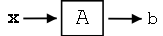
También podemos usar los vectores\(\left\{v_{1}, v_{2}, \ldots, v_{n}\right\}\) para representar la salida,\(\mathbf{b}\), de un sistema:
\[\mathbf{b}=A \mathbf{x}=A\left(\alpha_{1} v_{1}+\alpha_{2} v_{2}+\ldots+\alpha_{n} v_{n}\right) \nonumber \]
\[A \mathbf{x}=\alpha_{1} \lambda_{1} v_{1}+\alpha_{2} \lambda_{2} v_{2}+\ldots+\alpha_{n} \lambda_{n} v_{n}=\mathbf{b} \nonumber \]
\ [A x=\ left (\ begin {array} {cccc}
\ vdots &\ vdots &\ vdots\\
v_ {1} & v_ {2} &\ dots & v_ {n}\\ vdots &
\ vdots &\ vdots &\ vdots
\ end {array}\ right)\ left (\ begin {array} {c}
\ lambda_ {1}\ alpha_ {1}\\
\ vdots\\
\ lambda_ {1}\ alfa_ {n}
\ end {array}\ derecha)\ nonumber\]
\[A \mathbf{x}=V \Lambda \mathbf{\alpha} \nonumber \]
\[A \mathbf{x}=V \Lambda V^{-1} \mathbf{x} \nonumber \]
donde\(\Lambda\) está la matriz con los valores propios abajo de la diagonal:
\ [\ lambda=\ left (\ begin {array} {cccc}
\ lambda_ {1} & 0 &\ dots & 0\\
0 &\ lambda_ {2} &\ dots & 0\
\ dots &\ vdots &\ ddots &\ vdots &\ vdots\\
0 &\ dots &\ lambda_ {n}
\ end {array}\ right)\ nonumber \]
Finalmente, podemos cancelar el\(\mathbf{x}\) y se quedan con una ecuación final para\(A\):
\[A=V \Lambda V^{-1} \nonumber \]
Interpretación
Para nuestra interpretación, recuerde nuestras fórmulas clave:
\[\mathbf{\alpha}=V^{-1} \mathbf{x} \nonumber \]
\[b=\sum_{i} \alpha_{i} \lambda_{i} v_{i} \nonumber \]
Podemos interpretar operando\(\mathbf{x}\) con\(A\) como:
\ [\ izquierda (\ begin {array} {c}
x_ {1}\\
\ vdots\\
x_ {n}
\ end {array}\ derecha)\ derechafila\ izquierda (\ begin {array} {c}
\ alpha_ {1}\\ vdots
\\
\ alpha_ {n}
\ end {array}\ right)\ right)\ right tarrow\ left (\ begin {array} c {}
\ lambda_ {1}\ alpha_ {1}\\
\ vdots\
\ lambda_ {1}\ alpha_ {n}
\ end {array}\ derecha)\ derecha)\ fila derecha\ izquierda (\ begin {array} {c}
b_ {1}\
\ vdots\\
b_ {n}
\ end {array}\ derecha)\ nonumber\]
donde los tres pasos (flechas) de la ilustración anterior representan las siguientes tres operaciones:
- Transformar\(\mathbf{x}\) usando\(V^{-1}\), que rinde\(\alpha\)
- Multiplicación por\(\Lambda\)
- Transformación inversa usando\(V\), lo que nos da\(\mathbf{b}\)
¡Este es el paradigma que usaremos para los sistemas LTI!