1.7: Función de impulso de tiempo discreto

Última actualización
Guardar como PDF

Page ID: 86579

\( \newcommand{\vecs}[1]{\overset { \scriptstyle \rightharpoonup} {\mathbf{#1}} } \) \( \newcommand{\vecd}[1]{\overset{-\!-\!\rightharpoonup}{\vphantom{a}\smash {#1}}} \)\(\newcommand{\id}{\mathrm{id}}\) \( \newcommand{\Span}{\mathrm{span}}\) \( \newcommand{\kernel}{\mathrm{null}\,}\) \( \newcommand{\range}{\mathrm{range}\,}\) \( \newcommand{\RealPart}{\mathrm{Re}}\) \( \newcommand{\ImaginaryPart}{\mathrm{Im}}\) \( \newcommand{\Argument}{\mathrm{Arg}}\) \( \newcommand{\norm}[1]{\| #1 \|}\) \( \newcommand{\inner}[2]{\langle #1, #2 \rangle}\) \( \newcommand{\Span}{\mathrm{span}}\) \(\newcommand{\id}{\mathrm{id}}\) \( \newcommand{\Span}{\mathrm{span}}\) \( \newcommand{\kernel}{\mathrm{null}\,}\) \( \newcommand{\range}{\mathrm{range}\,}\) \( \newcommand{\RealPart}{\mathrm{Re}}\) \( \newcommand{\ImaginaryPart}{\mathrm{Im}}\) \( \newcommand{\Argument}{\mathrm{Arg}}\) \( \newcommand{\norm}[1]{\| #1 \|}\) \( \newcommand{\inner}[2]{\langle #1, #2 \rangle}\) \( \newcommand{\Span}{\mathrm{span}}\)\(\newcommand{\AA}{\unicode[.8,0]{x212B}}\)

Introducción

En ingeniería, a menudo nos ocupamos de la idea de que una acción ocurra en un momento determinado. Ya sea una fuerza en un punto en el espacio o alguna otra señal en un punto en el tiempo, vale la pena desarrollar alguna forma de definir cuantitativamente esto. Esto nos lleva a la idea de un impulso unitario, probablemente la segunda función más importante, junto a la compleja exponencial, en este curso de sistemas y señales.

Función de muestra de unidad

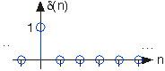
La función de muestra unitaria, a menudo conocida como la función de impulso unitario o delta, es la función que define la idea de un impulso unitario en tiempo discreto. No hay tantas complejidades involucradas en su definición como en la definición de la función delta de Dirac, la función de impulso de tiempo continuo. La función de muestra unitaria simplemente toma un valor de uno en\(n=0\) y un valor de cero en otra parte. La función de impulso a menudo se escribe como\(\delta[n]\).

\ [\ delta [n] =\ left\ {\ begin {array} {l}
1\ text {if} n=0\\
0\ text {de lo contrario}
\ end {array}\ right. \ nonumber\]

Figura\(\PageIndex{1}\): La muestra unitaria.

A continuación enumeraremos brevemente algunas propiedades importantes del impulso unitario sin entrar en detalle de sus pruebas.

Propiedades de Impulso de Unidad

\(\delta[n]=\delta[-n]\)
\(\delta[n]=u[n]-u[n-1]\)
\(x[n] \delta[n]=x[0] \delta[n]\)

\[\sum_{n=-\infty}^{\infty} x[n] \delta[n]=\sum_{n=-\infty}^{\infty} x[0] \delta[n]=x[0] \sum_{n=-\infty}^{\infty} \delta[n]=x[0] \nonumber \]

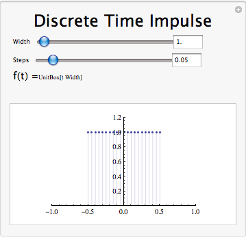
Demostración de respuesta de impulso de tiempo discreto

DTIdemo — Figura\(\PageIndex{2}\): Interactuar (cuando esté en línea) con un CDF de Mathematica demostrando la función de impulso de tiempo discreto.

Resumen de impulso de unidad de tiempo discreto

La función de impulso de unidad de tiempo discreta, también conocida como función de muestra unitaria, es de gran importancia para el estudio de señales y sistemas. La función toma un valor de uno a la vez\(n=0\) y un valor de cero en otra parte. Tiene varias propiedades importantes que volverán a aparecer al estudiar sistemas.