6.5: Promedios exponenciales y filtros recursivos
- Page ID
- 82421
\( \newcommand{\vecs}[1]{\overset { \scriptstyle \rightharpoonup} {\mathbf{#1}} } \)
\( \newcommand{\vecd}[1]{\overset{-\!-\!\rightharpoonup}{\vphantom{a}\smash {#1}}} \)
\( \newcommand{\id}{\mathrm{id}}\) \( \newcommand{\Span}{\mathrm{span}}\)
( \newcommand{\kernel}{\mathrm{null}\,}\) \( \newcommand{\range}{\mathrm{range}\,}\)
\( \newcommand{\RealPart}{\mathrm{Re}}\) \( \newcommand{\ImaginaryPart}{\mathrm{Im}}\)
\( \newcommand{\Argument}{\mathrm{Arg}}\) \( \newcommand{\norm}[1]{\| #1 \|}\)
\( \newcommand{\inner}[2]{\langle #1, #2 \rangle}\)
\( \newcommand{\Span}{\mathrm{span}}\)
\( \newcommand{\id}{\mathrm{id}}\)
\( \newcommand{\Span}{\mathrm{span}}\)
\( \newcommand{\kernel}{\mathrm{null}\,}\)
\( \newcommand{\range}{\mathrm{range}\,}\)
\( \newcommand{\RealPart}{\mathrm{Re}}\)
\( \newcommand{\ImaginaryPart}{\mathrm{Im}}\)
\( \newcommand{\Argument}{\mathrm{Arg}}\)
\( \newcommand{\norm}[1]{\| #1 \|}\)
\( \newcommand{\inner}[2]{\langle #1, #2 \rangle}\)
\( \newcommand{\Span}{\mathrm{span}}\) \( \newcommand{\AA}{\unicode[.8,0]{x212B}}\)
\( \newcommand{\vectorA}[1]{\vec{#1}} % arrow\)
\( \newcommand{\vectorAt}[1]{\vec{\text{#1}}} % arrow\)
\( \newcommand{\vectorB}[1]{\overset { \scriptstyle \rightharpoonup} {\mathbf{#1}} } \)
\( \newcommand{\vectorC}[1]{\textbf{#1}} \)
\( \newcommand{\vectorD}[1]{\overrightarrow{#1}} \)
\( \newcommand{\vectorDt}[1]{\overrightarrow{\text{#1}}} \)
\( \newcommand{\vectE}[1]{\overset{-\!-\!\rightharpoonup}{\vphantom{a}\smash{\mathbf {#1}}}} \)
\( \newcommand{\vecs}[1]{\overset { \scriptstyle \rightharpoonup} {\mathbf{#1}} } \)
\( \newcommand{\vecd}[1]{\overset{-\!-\!\rightharpoonup}{\vphantom{a}\smash {#1}}} \)
\(\newcommand{\avec}{\mathbf a}\) \(\newcommand{\bvec}{\mathbf b}\) \(\newcommand{\cvec}{\mathbf c}\) \(\newcommand{\dvec}{\mathbf d}\) \(\newcommand{\dtil}{\widetilde{\mathbf d}}\) \(\newcommand{\evec}{\mathbf e}\) \(\newcommand{\fvec}{\mathbf f}\) \(\newcommand{\nvec}{\mathbf n}\) \(\newcommand{\pvec}{\mathbf p}\) \(\newcommand{\qvec}{\mathbf q}\) \(\newcommand{\svec}{\mathbf s}\) \(\newcommand{\tvec}{\mathbf t}\) \(\newcommand{\uvec}{\mathbf u}\) \(\newcommand{\vvec}{\mathbf v}\) \(\newcommand{\wvec}{\mathbf w}\) \(\newcommand{\xvec}{\mathbf x}\) \(\newcommand{\yvec}{\mathbf y}\) \(\newcommand{\zvec}{\mathbf z}\) \(\newcommand{\rvec}{\mathbf r}\) \(\newcommand{\mvec}{\mathbf m}\) \(\newcommand{\zerovec}{\mathbf 0}\) \(\newcommand{\onevec}{\mathbf 1}\) \(\newcommand{\real}{\mathbb R}\) \(\newcommand{\twovec}[2]{\left[\begin{array}{r}#1 \\ #2 \end{array}\right]}\) \(\newcommand{\ctwovec}[2]{\left[\begin{array}{c}#1 \\ #2 \end{array}\right]}\) \(\newcommand{\threevec}[3]{\left[\begin{array}{r}#1 \\ #2 \\ #3 \end{array}\right]}\) \(\newcommand{\cthreevec}[3]{\left[\begin{array}{c}#1 \\ #2 \\ #3 \end{array}\right]}\) \(\newcommand{\fourvec}[4]{\left[\begin{array}{r}#1 \\ #2 \\ #3 \\ #4 \end{array}\right]}\) \(\newcommand{\cfourvec}[4]{\left[\begin{array}{c}#1 \\ #2 \\ #3 \\ #4 \end{array}\right]}\) \(\newcommand{\fivevec}[5]{\left[\begin{array}{r}#1 \\ #2 \\ #3 \\ #4 \\ #5 \\ \end{array}\right]}\) \(\newcommand{\cfivevec}[5]{\left[\begin{array}{c}#1 \\ #2 \\ #3 \\ #4 \\ #5 \\ \end{array}\right]}\) \(\newcommand{\mattwo}[4]{\left[\begin{array}{rr}#1 \amp #2 \\ #3 \amp #4 \\ \end{array}\right]}\) \(\newcommand{\laspan}[1]{\text{Span}\{#1\}}\) \(\newcommand{\bcal}{\cal B}\) \(\newcommand{\ccal}{\cal C}\) \(\newcommand{\scal}{\cal S}\) \(\newcommand{\wcal}{\cal W}\) \(\newcommand{\ecal}{\cal E}\) \(\newcommand{\coords}[2]{\left\{#1\right\}_{#2}}\) \(\newcommand{\gray}[1]{\color{gray}{#1}}\) \(\newcommand{\lgray}[1]{\color{lightgray}{#1}}\) \(\newcommand{\rank}{\operatorname{rank}}\) \(\newcommand{\row}{\text{Row}}\) \(\newcommand{\col}{\text{Col}}\) \(\renewcommand{\row}{\text{Row}}\) \(\newcommand{\nul}{\text{Nul}}\) \(\newcommand{\var}{\text{Var}}\) \(\newcommand{\corr}{\text{corr}}\) \(\newcommand{\len}[1]{\left|#1\right|}\) \(\newcommand{\bbar}{\overline{\bvec}}\) \(\newcommand{\bhat}{\widehat{\bvec}}\) \(\newcommand{\bperp}{\bvec^\perp}\) \(\newcommand{\xhat}{\widehat{\xvec}}\) \(\newcommand{\vhat}{\widehat{\vvec}}\) \(\newcommand{\uhat}{\widehat{\uvec}}\) \(\newcommand{\what}{\widehat{\wvec}}\) \(\newcommand{\Sighat}{\widehat{\Sigma}}\) \(\newcommand{\lt}{<}\) \(\newcommand{\gt}{>}\) \(\newcommand{\amp}{&}\) \(\definecolor{fillinmathshade}{gray}{0.9}\)Supongamos que intentamos extender nuestro método para calcular promedios móviles finitos a promedios móviles infinitos de la forma
\ [\ begin {align}
x_ {n} &=\ qquad\ qquad\ qquad\ suma_ {k=0} ^ {\ infty} w_ {k} u_ {n-k}\ nonumber\\
&=w_ {0} u_ {n} +w_ {1} u_ {n-1} +\ cdots+w_ {1000} u_ {n-1000} +\ cdots
\ end {align}\ nonumber\]
En general, esta media móvil requeriría memoria infinita para los coeficientes de ponderación\(w_{0}, w_{1}, \ldots\) y para las entradas\(u_{n}, u_{n-1}, \ldots\). Además, el hardware para multiplicar wkun−kwkun-k tendría que ser infinitamente rápido para calcular la media móvil infinita en tiempo finito. Todo esto es claramente fantasioso e inverosímil (sin mencionar imposible). Pero, ¿y si los pesos toman la forma exponencial
\[w_{k}= \begin{cases}0, & k<0 \\ w_{0} a^{k}, & k \geq 0 ?\end{cases} \nonumber \]
¿Algún resultado de simplificación? Hay esperanza porque la secuencia de ponderación obedece a la recursión
\[w_{k}= \begin{cases}0, & k<0 \\ w_{0}, & k=0 \\ a w_{k-1} & k \geq 1\end{cases} \nonumber \]
Esta recursión puede ser reescrita de la siguiente manera, para\(k \geq 1\):
\[w_{k}-a w_{k-1}=0, k \geq 1 \nonumber \]
Ahora manipulemos la media móvil infinita y utilicemos la recursión para los pesos para ver qué sucede. Debes seguir cada paso:
\ [\ begin {align}
x_ {n} &=\ suma_ {k=0} ^ {\ infty} w_ {k} u_ {n-k}\ nonumber\\
&=\ quad\ suma_ {k=1} ^ {\ infty} w_ {k} u_ {n-k} +w_ {0} u_ {n}\ nonúmero\\
&= _ {k=1} ^ {\ infty} a w_ {k-1} u_ {n-k} +w_ {0} u_ {n}\ nonumber\\
&=a\ suma_ {m=0} ^ {\ infty} w_ {m} u_ {n-1- m} +w_ {0} u_ {n}\ nonumber\\
&=a x_ {n-1} +w_ {0} u_ {n}.
\ end {align}\ nonumber\]
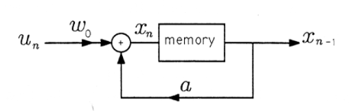
Este resultado es fundamentalmente importante porque dice que la salida de la media móvil exponencial infinita puede calcularse escalando la salida anterior\(x_{n-1}\) por la constante\(a\), escalando la nueva entrada\(u_n\) por\(w_0\), y sumando. Solo se deben asignar tres ubicaciones de memoria: una para\(w_0\), una para\(a\) y otra para\(x_{n-1}\). Sólo se deben implementar dos multiplicaciones: una para\(ax_{n-1}\) y otra para\(w_0u_n\). En la Figura 1 se da un diagrama de la recursión. En esta recursión, el antiguo valor de la media móvil exponencial\(x_{n-1}\),, se escala\(a\) y se suma\(w_0u_n\) para producir la nueva media móvil exponencial\(x_n\). Este nuevo valor se almacena en la memoria, donde se convierte\(x_{n-1}\) en el siguiente paso de la recursión, y así sucesivamente.

Intentar extender la recursión de los párrafos anteriores al promedio ponderado
\(x_{n}=\sum_{k=0}^{N-1} a^{k} u_{n-k} .\)
¿Qué sale mal?
Calcular la salida de la media móvil exponencial\(x_{n}=a x_{n-1}+w_{0} u_{n}\) cuando la entrada es
\(u_{n}= \begin{cases}0, & n<0 \\ u, & n \geq 0\end{cases}\)
Traza tu resultado versus\(n\).
Calcular\(w_0\) en la secuencia de ponderación exponencial
\(w_{n}= \begin{cases}0, & n<0 \\ a^{n} w_{0}, & n \geq 0\end{cases}\)
para que la secuencia de ponderación sea una ventana válida. (Este es un caso especial del Ejercicio 3 de Filtrado: Promedios Móviles.) Asumir\(−1<a<1\)