
1.3: Proyección Estereográfica
- Page ID
- 115630

Proyección estereográfica\(S^1\to \hat{\mathbb{R}}\)
Dejar\(S^1\) denotar el círculo unitario en el\(x,y\) plano -plano.
\ [
S^1 =\ {(x, y)\ in\ mathbb {R} ^2\ dos puntos x^2+y^2=1\}\ etiqueta {s1defn}\ etiqueta {1.3.1}
\]
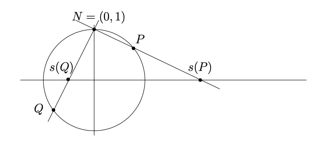
Dejar\(N=(0,1)\) denotar el “polo norte” (es decir, el punto en la “parte superior” del círculo unitario). Dado un punto\(P=(x,y)\neq N\) en el círculo unitario, vamos a\(s(P)\) denotar la intersección de la línea\(\overline{NP}\) con el\(x\) eje -eje. Ver Figura 1.3.1. El mapa\(s\colon S^1\setminus \{N\}\to \mathbb{R}\) dado por esta regla se denomina proyección estereográfica. Usando triángulos similares, es fácil ver que\(s(x,y)=\frac{x}{1-y}\text{.}\)
- Punto de control 1.3.2.
-
Dibuja los triángulos similares relevantes y verifica la fórmula\(s(x,y) = \frac{x}{1-y}\text{.}\)
Extendemos la proyección estereográfica a todo el círculo unitario de la siguiente manera. Llamamos al conjunto
\[\hat{\mathbb{R}}=\mathbb{R}\cup \{\infty\}\label{extendedrealsdefn}\tag{1.3.2}\]
los números reales extendidos, donde\(∞\) "" es un elemento que no es un número real. Ahora definimos proyección estereográfica\(s\colon S^1 \to \hat{\mathbb{R}}\) por\ [s (x, y) =\ left\ {
\ begin {array} {cc}
\ frac {x} {1-y} & y\ neq 1\\
\ infty & y=1
\ end {array}
\ derecha.. \ label {stereoproj1defn}\ tag {1.3.3}\]
Proyección estereográfica\(S^2\to \hat{\mathbb{C}}\)
Las definiciones de la subsección anterior se extienden naturalmente a dimensiones superiores. Aquí están los detalles para el caso principal de interés.
Dejar\(S^2\) denotar la esfera de la unidad en\(\mathbb{R}^3\text{.}\)
\ [
S^2 =\ {(a, b, c)\ in\ mathbb {R} ^3\ colon a^2+b^2+c^2=1\}\ etiqueta {s2defn}\ tag {1.3.4}
\]
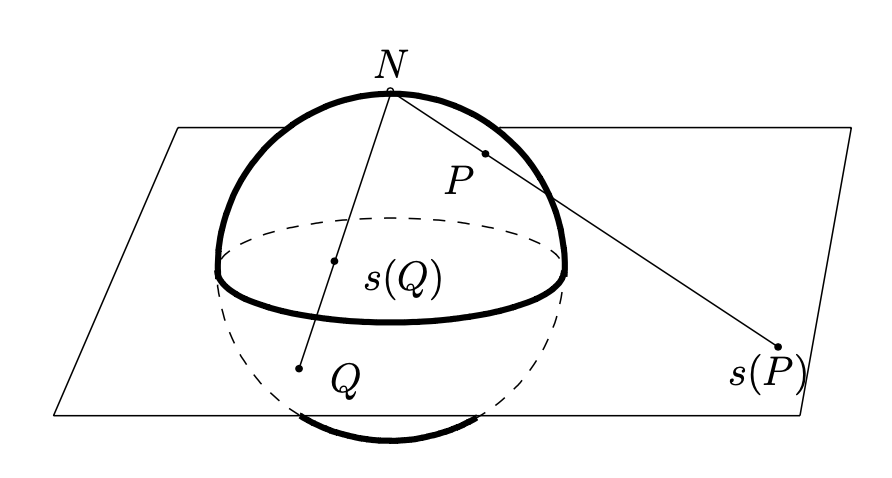
Dejar\(N=(0,0,1)\) denotar el “polo norte” (es decir, el punto en la “parte superior” de la esfera, donde el\(z\) eje positivo es “arriba”). Dado un punto\(P=(a,b,c)\neq N\) en la esfera unitaria, vamos a\(s(P)\) denotar la intersección de la línea\(\overline{NP}\) con el\(x,y\) -plano, que identificamos con el plano complejo\(\mathbb{C}\). Ver Figura 1.3.3. El mapa\(s\colon S^2\setminus \{N\}\to \mathbb{C}\) dado por esta regla se denomina proyección estereográfica. Usando triángulos similares, es fácil ver que\(s(a,b,c)=\frac{a+ib}{1-c}\text{.}\)
Extendemos la proyección estereográfica a toda la esfera unitaria de la siguiente manera. Llamamos al conjunto
\[\hat{\mathbb{C}}=\mathbb{C}\cup \{\infty\}\label{extendedcomplexsdefn}\tag{1.3.5}\]
los números complejos extendidos, donde\(∞\) "" es un elemento que no es un número complejo. Ahora definimos proyección estereográfica\(s\colon S^2 \to \hat{\mathbb{C}}\) por
\ [s (a, b, c) =\ izquierda\ {
\ begin {array} {cc}
\ frac {a+ib} {1-c} & c\ neq 1\\
\ infty & c=1
\ end {array}
\ derecha.. \ label {stereoprojdefn}\ tag {1.3.6}
\]
Ejercicios
Fórmulas para proyección estereográfica inversa.
Es intuitivamente claro que la proyección estereográfica es una bijección. Haz esto riguroso encontrando una fórmula para lo inverso.
Para\(s\colon S^1\to \hat{\mathbb{R}}\text{,}\) encontrar una fórmula para\(s^{-1}\colon \hat{\mathbb{R}}\to S^1\text{.}\) Find\(s^{-1}(3)\text{.}\)
- Contestar
-
\ [
s^ {-1} (r) =\ comenzar {casos}
\ izquierda (\ frac {2r} {r^2+1},\ frac {r^2-1} {r^2+1}\ derecha) &
\ texto {si} r\ neq\ infty\ (0,1) &\ text {si} r=\ infty
\ end {casos}
\ nonumber\]\(s^{-1}(3) = (3/5,4/5)\)
Para\(s\colon S^2\to \hat{\mathbb{C}}\text{,}\) encontrar una fórmula para\(s^{-1}\colon \hat{\mathbb{C}}\to S^2\text{.}\) Find\(s^{-1}(3+i)\text{.}\)
- Contestar
-
\ [
s^ {-1} (z) =\ comenzar {casos}
\ izquierda (\ frac {2Re (z)} {|z|^2+1},\ frac {2Im (z)} {|z|^2+1},
\ frac {|z|^2-1} {|z|^2+1}\ derecha) &\ text {si} z\ neq
\ infty\ (0,0,1) &\ texto {si} z=\ infty\ fin {casos}
\ nonumber\]\(s^{-1}(3+i) = (6/11,2/11,9/11)\)
Transformaciones conjugadas.
Dejar\(\mu \colon X\to Y\) ser un mapa biyective. Decimos que los mapas y\(f\colon X\to X\) y\(g\colon Y\to Y\) son transformaciones conjugadas (con respecto a la biyección\(\mu\)) si\(f = \mu^{-1}\circ g\circ \mu\text{.}\)
Mostrar que los mapas\(S^1\to S^1\) dados por\((x,y)\to (x,-y)\) y\(\hat{\mathbb{R}}\to \hat{\mathbb{R}}\) dados por\(x\to 1/x\) son transformaciones conjugadas con respecto a la proyección estereográfica
Mostrar que el mapa\(R_{Z,\theta}\colon S^2\to S^2\) dado por\ ((a, b, c)\ to
(a\ cos\ theta-b\ sin\ theta, a\ sin\ theta+b\ cos\ theta, c)\) (una rotación alrededor del\(z\) -eje por ángulo\(θ\)) y el mapa\(T_{Z,\theta}\colon \hat{\mathbb{C}}\to \hat{\mathbb{C}}\) dado por\(z\to e^{i\theta}z\) son transformaciones conjugadas con respecto a la proyección estereográfica.
Mostrar que el mapa\(R_{X,\pi}\colon S^2\to S^2\) dado por\((a,b,c)\to (a,-b,-c)\) (rotación alrededor del\(x\) eje por\(\pi\) radianes) y el mapa\(T_{X,\pi}\colon \hat{\mathbb{C}}\to \hat{\mathbb{C}}\) dado por\(z\to 1/z\) son transformaciones conjugadas con respecto a la proyección estereográfica.
Mostrar que el mapa\(R_{X,\pi/2}\colon S^2\to S^2\) dado por\((a,b,c)\to (a,-c,b)\) (rotación alrededor del\(x\) eje por\(\pi/2\) radianes) y el mapa\(T_{X,\pi/2}\colon \hat{\mathbb{C}}\to \hat{\mathbb{C}}\) dado por\(z\to \frac{z+i}{iz+1}\) son transformaciones conjugadas con respecto a la proyección estereográfica.
7. Proyecciones de extremos de diámetros.
Demostrar que\(s(a,b,c)(s(-a,-b,-c))^\ast=-1\) para cualquier punto\((a,b,c)\) en\(S^2\) con\(|c|\neq 1\text{.}\) Inversamente, supongamos que\(zw^\ast=-1\) para algunos\(z,w\in \mathbb{C}\text{.}\) Mostrar eso.