6.7: Funciones inversas e implícitas. Mapas abiertos y cerrados

I. “Si\(f \in C D^{1}\) en\(\vec{p},\) ese entonces\(f\) se asemeja a un mapa lineal (es decir,\(d f )\) en\(\vec{p}."\) Persiguiendo esta idea básica, primero hacemos precisa nuestra noción de"\(f \in C D^{1}\) at\(\vec{p}\).”

Definición 1

Un mapa\(f : E^{\prime} \rightarrow E\) es continuamente diferenciable, o de clase\(C D^{1}\) (escrito\(f \in C D^{1}),\) en\(\vec{p}\) iff la siguiente declaración es verdadera:

\[\begin{array}{l}{\text { Given any } \varepsilon>0, \text { there is } \delta>0 \text { such that } f \text { is differentiable on the }} \\ {\text { globe } \overline{G}=\overline{G_{\vec{p}}(\delta)}, \text { with }} \\ {\qquad\|d f(\vec{x} ; \cdot)-d f(\vec{p} ; \cdot)\|<\varepsilon \text { for all } \vec{x} \in \overline{G}.}\end{array}\]

Por Problema 10 en §5, esta definición concuerda con la Definición 1 §5, pero ya no se limita al caso\(E^{\prime}=E^{n}\left(C^{n}\right).\) Ver también Problemas 1 y 2 a continuación.

Ahora obtenemos el siguiente resultado.

Teorema\(\PageIndex{1}\)

Dejar\(E^{\prime}\) y\(E\) estar completo. Si\(f : E^{\prime} \rightarrow E\) es de clase\(C D^{1}\) en\(\vec{p}\) y si\(d f(\vec{p} ; \cdot)\) es biyective (§6), entonces\(f\) es uno a uno en algún globo\(\overline{G}=\overline{G_{\vec{p}}}(\delta).\)

Así\(f\) “localmente” se asemeja a df\((\vec{p} ; \cdot)\) en este sentido.

Prueba

Set\(\phi=d f(\vec{p} ; \cdot)\) y

\[\left\|\phi^{-1}\right\|=\frac{1}{\varepsilon}\]

(cf. Teorema 2 del §6).

Por Definición 1, arreglar\(\delta>0\) para que para\(\vec{x} \in \overline{G}=\overline{G_{\vec{p}}(\delta)}\).

\[\|d f(\vec{x} ; \cdot)-\phi\|<\frac{1}{2} \varepsilon.\]

Luego por la Nota 5 en §2,

\[(\forall \vec{x} \in \overline{G})\left(\forall \vec{u} \in E^{\prime}\right) \quad|d f(\vec{x} ; \vec{u})-\phi(\vec{u})| \leq \frac{1}{2} \varepsilon|\vec{u}|.\]

Ahora arregla cualquiera\(\vec{r}, \vec{s} \in \overline{G}, \vec{r} \neq \vec{s},\) y establece\(\vec{u}=\vec{r}-\vec{s} \neq 0.\) De nuevo, por la Nota 5 en §2,

\[|\vec{u}|=\left|\phi^{-1}(\phi(\vec{u}))\right| \leq\left\|\phi^{-1}\right\||\phi(\vec{u})|=\frac{1}{\varepsilon}|\phi(\vec{u})|;\]

por lo

\[0<\varepsilon|\vec{u}| \leq|\phi(\vec{u})|.\]

Por convexidad,\(\overline{G} \supseteq I=L[\vec{s}, \vec{r}],\) entonces (1) se sostiene para\(\vec{x} \in I, \vec{x}=\vec{s}+t \vec{u}, 0 \leq t \leq 1\).

Al señalar esto, establecer

\[h(t)=f(\vec{s}+t \vec{u})-t \phi(\vec{u}), \quad t \in E^{1}.\]

Entonces para\(0 \leq t \leq 1\),

\[\begin{aligned} h^{\prime}(t) &=D_{\vec{u}} f(\vec{s}+t \vec{u})-\phi(\vec{u}) \\ &=d f(\vec{s}+t \vec{u} ; \vec{u})-\phi(\vec{u}). \end{aligned}\]

(¡Verifica!) Así, por (1) y (2),

\[\begin{aligned} \sup _{0 \leq t \leq 1}\left|h^{\prime}(t)\right| &=\sup _{0 \leq t \leq 1}|d f(\vec{s}+t \vec{u} ; \vec{u})-\phi(\vec{u})| \\ & \leq \frac{\varepsilon}{2}|\vec{u}| \leq \frac{1}{2}|\phi(\vec{u})|. \end{aligned}\]

(¡Explique!) Ahora, por Corolario 1 en el Capítulo 5, §4,

\[|h(1)-h(0)| \leq(1-0) \cdot \sup _{0 \leq t \leq 1}\left|h^{\prime}(t)\right| \leq \frac{1}{2}|\phi(\vec{u})|.\]

Como\(h(0)=f(\vec{s})\) y

\[h(1)=f(\vec{s}+\vec{u})-\phi(\vec{u})=f(\vec{r})-\phi(\vec{u}),\]

obtenemos (incluso si\(\vec{r}=\vec{s})\)

\[|f(\vec{r})-f(\vec{s})-\phi(\vec{u})| \leq \frac{1}{2}|\phi(\vec{u})| \quad(\vec{r}, \vec{s} \in \overline{G}, \vec{u}=\vec{r}-\vec{s}).\]

Pero por la ley del triángulo,

\[|\phi(\vec{u})|-|f(\vec{r})-f(\vec{s})| \leq|f(\vec{r})-f(\vec{s})-\phi(\vec{u})|.\]

Por lo tanto

\[|f(\vec{r})-f(\vec{s})| \geq \frac{1}{2}|\phi(\vec{u})| \geq \frac{1}{2} \varepsilon|\vec{u}|=\frac{1}{2} \varepsilon|\vec{r}-\vec{s}|\]

por (2).

De ahí\(f(\vec{r}) \neq f(\vec{s})\) que siempre\(\overline{G};\) que\(\vec{r} \neq \vec{s}\) en así\(f\) sea uno a uno encendido\(\overline{G},\) como se reclama. \(\quad \square\)

Corolario\(\PageIndex{1}\)

Bajo los supuestos del Teorema 1, los mapas\(f\) y\(f^{-1}\) (el inverso de\(f\) restringido a\(\overline{G}\)) son uniformemente continuos sobre\(\overline{G}\) y\(f[\overline{G}],\) respectivamente.

Prueba

Por (3),

\[\begin{aligned}|f(\vec{r})-f(\vec{s})| & \leq|\phi(\vec{u})|+\frac{1}{2}|\phi(\vec{u})| \\ & \leq|2 \phi(\vec{u})| \\ & \leq 2\|\phi\||\vec{u}| \\ &=2\|\phi\||\vec{r}-\vec{s}| \quad(\vec{r}, \vec{s} \in \overline{G}). \end{aligned}\]

Esto implica una continuidad uniforme para\(f\). (¿Por qué?)

A continuación,\(g=f^{-1}\) vamos\(H=f[\overline{G}]\).

Si se\(\vec{x}, \vec{y} \in H,\) deja\(\vec{r}=g(\vec{x})\) y\(\vec{s}=g(\vec{y});\) así\(\vec{r}, \vec{s} \in \overline{G},\) con\(\vec{x}=f(\vec{r})\) y\(\vec{y}=f(\vec{s}).\) Por lo tanto por (4),

\[|\vec{x}-\vec{y}| \geq \frac{1}{2} \varepsilon|g(\vec{x})-g(\vec{y})|,\]

demostrando todo para\(g,\) también. \(\quad \square\)

Nuevamente,\(f\) se asemeja a\(\phi\) lo que es uniformemente continuo, junto con\(\phi^{-1}\).

II. Introducimos la siguiente definición.

Definición 2

Un mapa\(f :(S, \rho) \rightarrow\left(T, \rho^{\prime}\right)\) está cerrado (abierto) en\(D \subseteq S\) iff, para cualquier\(X \subseteq D\) el conjunto\(f[X]\) está cerrado (abierto) en\(T\) siempre que\(X\) sea así en\(S.\)

Tenga en cuenta que los mapas continuos tienen tal propiedad para imágenes inversas (Problema 15 en el Capítulo 4, §2).

Corolario\(\PageIndex{2}\)

Bajo los supuestos del Teorema 1,\(f\) se cierra\(\overline{G},\) y así el conjunto\(f[\overline{G}]\) se cierra en\(E.\)

De manera similar para el mapa\(f^{-1}\) en\(f[\overline{G}]\).

Prueba para\(E^{\prime}=E=E^{n}\left(C^{n}\right)\) (para el caso general, ver Problema 6)

Dado cualquier cerrado\(X \subseteq \overline{G},\) debemos mostrar que\(f[X]\) está cerrado en\(E.\)

Ahora, como\(\overline{G}\) está cerrado y acotado, es compacto (Teorema 4 del Capítulo 4, §6).

Así también lo es\(X\) (Teorema 1 en el Capítulo 4, §6), y así es\(f[X]\) (Teorema 1 del Capítulo 4, §8).

Por Teorema 2 en el Capítulo 4, §6,\(f[X]\) se cierra, según se requiera. \(\quad \square\)

Para el resto de esta sección, estableceremos\(E^{\prime}=E=E^{n}\left(C^{n}\right)\).

Teorema\(\PageIndex{2}\)

Si\(E^{\prime}=E=E^{n}\left(C^{n}\right)\) en el Teorema 1, con otros supuestos sin cambios, entonces\(f\) está abierto en el globo\(G=G_{\vec{p}}(\delta),\) con\(\delta\) lo suficientemente pequeño.

Prueba

Primero probamos el siguiente lema.

Lema

\(f[G]\)contiene un globo\(G_{\vec{q}}(\alpha)\) donde\(\vec{q}=f(\vec{p})\).

Prueba

En efecto, vamos

\[\alpha=\frac{1}{4} \varepsilon \delta,\]

donde\(\delta\) y\(\varepsilon\) son como en la prueba del Teorema 1. (Seguimos la notación y fórmulas de esa prueba.)

Arreglar cualquier\(\vec{c} \in G_{\vec{q}}(\alpha);\)

\[|\vec{c}-\vec{q}|<\alpha=\frac{1}{4} \varepsilon \delta.\]

Establecer\(h=|f-\vec{c}|\)\(E^{\prime}.\) como\(f\) es uniformemente continuo en\(\overline{G},\) así es\(h\).

Ahora bien,\(\overline{G}\) es compacto en el\(E^{n}\left(C^{n}\right);\) Teorema 2 (ii) en el Capítulo 4, §8, rinde un punto\(\vec{r} \in \overline{G}\) tal que

\[h(\vec{r})=\min h[\overline{G}].\]

Afirmamos que\(\vec{r}\) está en\(G\) (el interior de\(\overline{G})\).

De lo contrario,\(|\vec{r}-\vec{p}|=\delta ;\) para por (4),

\[\begin{aligned} 2 \alpha=\frac{1}{2} \varepsilon \delta=\frac{1}{2} \varepsilon|\vec{r}-\vec{p}| & \leq|f(\vec{r})-f(\vec{p})| \\ & \leq|f(\vec{r})-\vec{c}|+|\vec{c}-f(\vec{p})| \\ &=h(\vec{r})+h(\vec{p}). \end{aligned}\]

Pero

\[h(\vec{p})=|\vec{c}-f(\vec{p})|=|\vec{c}-\vec{q}|<\alpha;\]

y así (7) rinde

\[h(\vec{p})<\alpha<h(\vec{r}),\]

contrario a la minimalidad de\(h(\vec{r})\) (ver (6)). Así\(|\vec{r}-\vec{p}|\) no puede igualar\(\delta\).

Lo\(f(\vec{r}) \in f[G].\) obtenemos\(\vec{r} \in G_{\vec{p}}(\delta)=G\) y\(|\vec{r}-\vec{p}|<\delta,\) ahora demostraremos que\(\vec{c}=f(\vec{r}).\)

Para ello, nos fijamos\(\vec{v}=\vec{c}-f(\vec{r})\) y demostramos que\(\vec{v}=\overrightarrow{0}.\) Let

\[\vec{u}=\phi^{-1}(\vec{v}),\]

donde

\[\phi=d f(\vec{p} ; \cdot),\]

como antes. Entonces

\[\vec{v}=\phi(\vec{u})=d f(\vec{p} ; \vec{u}).\]

Con\(\vec{r}\) lo anterior, arregle algunos

\[\vec{s}=\vec{r}+t \vec{u} \quad(0<t<1)\]

con\(t\) tan pequeño que\(\vec{s} \in G\) también. Luego por la fórmula (3),

\[|f(\vec{s})-f(\vec{r})-\phi(t \vec{u})| \leq \frac{1}{2}|t \vec{v}|;\]

también,

\[|f(\vec{r})-\vec{c}+\phi(t \vec{u})|=(1-t)|\vec{v}|=(1-t) h(\vec{r})\]

por nuestra elección de\(\vec{v}, \vec{u}\) y por\(h.\) lo tanto por la ley del triángulo,

\[h(\vec{s})=|f(\vec{s})-\vec{c}| \leq\left(1-\frac{1}{2} t\right) h(\vec{r}).\]

(¡Verifica!)

Como\(0<t<1,\) esto implica\(h(\vec{r})=0\) (de lo contrario,\(h(\vec{s})<h(\vec{r}),\) violar (6)).

Así, de hecho,

\[|\vec{v}|=|f(\vec{r})-\vec{c}|=0,\]

es decir,

\[\vec{c}=f(\vec{r}) \in f[G] \quad \text { for } \vec{r} \in G.\]

Pero\(\vec{c}\) fue un punto arbitrario de\(G_{\vec{q}}(\alpha).\) Por lo tanto

\[G_{\vec{q}}(\alpha) \subseteq f[G],\]

demostrando el lema. \(\quad \square\)

Prueba de Teorema 2. El lema muestra que\(f(\vec{p})\) está en el interior de\(f[G]\) si\(\vec{p}, f, d f(\vec{p} ; \cdot),\) y\(\delta\) son como en el Teorema 1.

Pero la Definición 1 implica que aquí\(f \in C D^{1}\) en todos\(G\) (ver Problema 1).

También,\(d f(\vec{x} ; \cdot)\) es biyectiva para cualquiera\(\vec{x} \in G\) por nuestra elección de\(G\) y Teoremas 1 y 2 en §6.

Por lo tanto,\(f\) mapea todo\(\vec{x} \in G\) en puntos interiores de,\(f[G];\) es decir,\(f\) mapea cualquier conjunto abierto\(X \subseteq G\) en un abierto\(f[X],\) según sea necesario. \(\quad \square\)

Nota 1. Un mapa

\[f :(S, \rho) \underset{\text { onto }}{\longleftrightarrow} (T, \rho^{\prime})\]

es tanto abierto como cerrado (“clopen”) iff\(f^{-1}\) es continuo - ver Problema 15 (iv) (v) en el Capítulo 4, §2, intercambiable\(f\) y\(f^{-1}.\)

Así\(\phi=d f(\vec{p} ; \cdot)\) en Teorema 1 es “clopen” en todos\(E^{\prime}\).

Nuevamente,\(f\) localmente se parece\(d f(\vec{p} ; \cdot)\).

III. El Teorema de la Función Inversa. Ahora seguimos persiguiendo estas ideas.

Teorema\(\PageIndex{3}\) (inverse functions)

Bajo los supuestos del Teorema 2, deja\(g\) ser la inversa de\(f_{G}\left(f \text { restricted to } G=G_{\vec{p}}(\delta)\right)\).

Entonces\(g \in C D^{1}\) encendido\(f[G]\) y\(d g(\vec{y} ; \cdot)\) es la inversa de\(d f(\vec{x} ; \cdot)\) siempre\(\vec{x}=g(\vec{y}), \vec{x} \in G.\)

Brevemente: “El diferencial de lo inverso es el inverso del diferencial”.

Prueba

Fijar cualquier\(\vec{y} \in f[G]\) y\(\vec{x}=g(\vec{y}) ;\) así\(\vec{y}=f(\vec{x})\) y\(\vec{x} \in G.\) dejar\(U=d f(\vec{x} ; \cdot).\)

Como se señaló anteriormente,\(U\) es biyectiva para cada uno\(\vec{x} \in G\) por los Teoremas 1 y 2 en §6; así\(V=U^{-1}.\) podremos establecer Debemos demostrar que\(V=d g(\vec{y} ; \cdot).\)

Para ello, da\(\vec{y}\) un incremento arbitrario (variable)\(\Delta \vec{y},\) tan pequeño que\(\vec{y}+\Delta \vec{y}\) permanezca en\(f[G]\) (un conjunto abierto por el Teorema 2).

Como\(g\) y\(f_{G}\) son uno a uno, determina de\(\Delta \vec{y}\) manera única

\[\Delta \vec{x}=g(\vec{y}+\Delta \vec{y})-g(\vec{y})=\vec{t},\]

y viceversa:

\[\Delta \vec{y}=f(\vec{x}+\vec{t})-f(\vec{x}).\]

Aquí\(\Delta \vec{y}\) y\(\vec{t}\) están los incrementos mutuamente correspondientes de\(\vec{y}=f(\vec{x})\) y\(\vec{x}=g(\vec{y}).\) Por continuidad,\(\vec{y} \rightarrow \overrightarrow{0}\) iff\(\vec{t} \rightarrow \overrightarrow{0}.\)

Como\(U=d f(\vec{x} ; \cdot)\),

\[\lim _{\vec{t} \rightarrow \overline{0}} \frac{1}{|\vec{t}|}|f(\vec{x}+\vec{t})-f(\vec{t})-U(\vec{t})|=0,\]

o

\[\lim _{\vec{t} \rightarrow \overrightarrow{0}} \frac{1}{|\vec{t}|}|F(\vec{t})|=0,\]

donde

\[F(\vec{t})=f(\vec{x}+\vec{t})-f(\vec{t})-U(\vec{t}).\]

Como\(V=U^{-1},\) tenemos

\[V(U(\vec{t}))=\vec{t}=g(\vec{y}+\Delta \vec{y})-g(\vec{y}).\]

Así que a partir de (9),

\[\begin{aligned} V(F(\vec{t})) &=V(\Delta \vec{y})-\vec{t} \\ &=V(\Delta \vec{y})-[g(\vec{y}+\Delta \vec{y})-g(\vec{y})]; \end{aligned}\]

es decir,

\[\frac{1}{|\Delta \vec{y}|}|g(\vec{y}+\Delta \vec{y})-g(\vec{y})-V(\Delta \vec{y})|=\frac{|V(F(\vec{t}))|}{|\Delta \vec{y}|}, \quad \Delta \vec{y} \neq \overrightarrow{0}.\]

Ahora, la fórmula (4), con\(\vec{r}=\vec{x}, \vec{s}=\vec{x}+\vec{t},\) y\(\vec{u}=\vec{t},\) muestra que

\[|f(\vec{x}+\vec{t})-f(\vec{x})| \geq \frac{1}{2} \varepsilon|\vec{t}|;\]

es decir,\(|\Delta \vec{y}| \geq \frac{1}{2} \varepsilon|\vec{t}|.\) Por lo tanto por (8),

\[\frac{|V(F(\vec{t}))|}{|\Delta \vec{y}|} \leq \frac{|V(F(\vec{t}) |}{\frac{1}{2} \varepsilon|\vec{t}|}=\frac{2}{\varepsilon}\left|V\left(\frac{1}{|\vec{t}|} F(\vec{t})\right)\right| \leq \frac{2}{\varepsilon}\|V\| \frac{1}{|\vec{t}|}|F(\vec{t})| \rightarrow 0 \text { as } \vec{t} \rightarrow \overrightarrow{0}.\]

Desde\(\vec{t} \rightarrow \overrightarrow{0}\) as\(\Delta \vec{y} \rightarrow \overrightarrow{0}\) (¡cambio de variables!) , la expresión (10) tiende a 0 como\(\Delta \vec{y} \rightarrow \overrightarrow{0}.\)

Por definición, entonces,\(g\) es diferenciable en\(\vec{y},\) con\(d g(\vec{y};)=V=U^{-1}\).

Por otra parte, aquí se aplica el Corolario 3 en §6. Por lo tanto

\[\left(\forall \delta^{\prime}>0\right)\left(\exists \delta^{\prime \prime}>0\right) \quad\|U-W\|<\delta^{\prime \prime} \Rightarrow\left\|U^{-1}-W^{-1}\right\|<\delta^{\prime}.\]

Tomando aquí\(U^{-1}=d g(\vec{y})\) y\(W^{-1}=d g(\vec{y}+\Delta \vec{y}),\) vemos que\(g \in C D^{1}\) cerca\(\vec{y}.\) Esto completa la prueba. \(\quad \square\)

Nota 2. Si\(E^{\prime}=E=E^{n}\left(C^{n}\right),\) la biyectividad de\(\phi=d f(\vec{p} ; \cdot)\) es equivalente a

\[\operatorname{det}[\phi]=\operatorname{det}\left[f^{\prime}(\vec{p})\right] \neq 0\]

(Teorema 1 de §6).

En este caso, el hecho de que\(f\) es uno-a-uno en\(G=G_{\vec{p}}(\delta)\) medio, componentwise (ver Nota 3 en §6), que el sistema de\(n\) ecuaciones

\[f_{i}(\vec{x})=f\left(x_{1}, \ldots, x_{n}\right)=y_{i}, \quad i=1, \ldots, n,\]

tiene una solución única para las\(n\)\(x_{k}\) incógnitas siempre y cuando

\[\left(y_{1}, \ldots, y_{n}\right)=\vec{y} \in f[G].\]

El teorema 3 muestra que esta solución tiene la forma

\[x_{k}=g_{k}(\vec{y}), \quad k=1, \ldots, n,\]

donde los\(g_{k}\) son de clase\(C D^{1}\) en\(f[G]\) siempre que\(f_{i}\) sean de clase\(C D^{1}\) cerca\(\vec{p}\) y det\(\left[f^{\prime}(\vec{p})\right] \neq 0.\) Aquí

\[\operatorname{det}\left[f^{\prime}(\vec{p})\right]=J_{f}(\vec{p}),\]

como en §6.

Así de nuevo\(f\) “localmente” se asemeja a un mapa lineal,\(\phi=d f(\vec{p} ; \cdot)\).

IV. El Teorema de la Función Implícita. Generalizando, ahora nos preguntamos, ¿qué pasa con resolver\(n\) ecuaciones en\(n+m\) incógnitas\(x_{1}, \ldots, x_{n}, y_{1}, \ldots, y_{m}?\) Decir, queremos resolver

\[f_{k}\left(x_{1}, \ldots, x_{n}, y_{1}, \ldots, y_{m}\right)=0, \quad k=1,2, \ldots, n,\]

para las primeras\(n\) incógnitas (o variables) expresándolas\(x_{k},\) así como

\[x_{k}=H_{k}\left(y_{1}, \ldots, y_{m}\right), \quad k=1, \ldots, n,\]

con\(H_{k} : E^{m} \rightarrow E^{1}\) o\(H_{k} : C^{m} \rightarrow C\).

Vamos a establecer\(\vec{x}=\left(x_{1}, \ldots, x_{n}\right), \vec{y}=\left(y_{1}, \ldots, y_{m}\right),\) y

\[(\vec{x}, \vec{y})=\left(x_{1}, \ldots, x_{n}, y_{1}, \ldots, y_{m}\right)\]

para que\((\vec{x}, \vec{y}) \in E^{n+m}\left(C^{n+m}\right)\).

Así, el sistema de ecuaciones (11) simplifica a

\[f_{k}(\vec{x}, \vec{y})=0, \quad k=1, \ldots, n\]

o

\[f(\vec{x}, \vec{y})=\overrightarrow{0},\]

donde\(f=\left(f_{1}, \ldots, f_{n}\right)\) es un mapa de\(E^{n+m}\left(C^{n+m}\right)\) into\(E^{n}\left(C^{n}\right) ; f\) es una función de\(n+m\) variables, pero tiene\(n\) componentes\(f_{k};\) i.e.

\[f(\vec{x}, \vec{y})=f\left(x_{1}, \ldots, x_{n}, y_{1}, \ldots, y_{m}\right)\]

es un vector en\(E^{n}\left(C^{n}\right)\).

Teorema\(\PageIndex{4}\) (implicit functions)

Let\(E^{\prime}=E^{n+m}\left(C^{n+m}\right), E=E^{n}\left(C^{n}\right),\) y let\(f : E^{\prime} \rightarrow E\) ser de clase\(C D^{1}\) cerca

\[(\vec{p}, \vec{q})=\left(p_{1}, \ldots, p_{n}, q_{1}, \ldots, q_{m}\right), \quad \vec{p} \in E^{n}\left(C^{n}\right), \vec{q} \in E^{m}\left(C^{m}\right).\]

Deja\([\phi]\) ser la\(n \times n\) matriz

\[\left(D_{j} f_{k}(\vec{p}, \vec{q})\right), \quad j, k=1, \ldots, n.\]

Si\(\operatorname{det}[\phi] \neq 0\) y si\(f(\vec{p}, \vec{q})=\overrightarrow{0},\) entonces hay conjuntos abiertos

\[P \subseteq E^{n}\left(C^{n}\right) \text { and } Q \subseteq E^{m}\left(C^{m}\right),\]

con\(\vec{p} \in P\) y\(\vec{q} \in Q,\) para el que hay un mapa único

\[H : Q \rightarrow P\]

con

\[f(H(\vec{y}), \vec{y})=\overrightarrow{0}\]

para todos\(\vec{y} \in Q;\) además,\(H \in C D^{1}\) en\(Q\).

Así\(\vec{x}=H(\vec{y})\) es una solución de (11) en forma de vector.

Prueba

Con la notación anterior, establezca

\[F(\vec{x}, \vec{y})=(f(\vec{x}, \vec{y}), \vec{y}), \quad F : E^{\prime} \rightarrow E^{\prime}.\]

Entonces

\[F(\vec{p}, \vec{q})=(f(\vec{p}, \vec{q}), \vec{q})=(\overrightarrow{0}, \vec{q}),\]

ya que\(f(\vec{p}, \vec{q})=\overrightarrow{0}\).

\((\vec{p}, \vec{q}),\)Tan\(f \in C D^{1}\) cerca como está\(F\) (verificar componentwise vía Problema 9 (ii) en §3 y Definición 1 de §5).

Por Teorema 4, §3,\(\operatorname{det}\left[F^{\prime}(\vec{p}, \vec{q})\right]=\operatorname{det}[\phi] \neq 0\) (¡explique!).

Así Teorema 1 anterior muestra que\(F\) es uno a uno en algún globo\(G\) sobre\((\vec{p}, \vec{q}).\)

Claramente\(G\) contiene un intervalo abierto sobre\((\vec{p}, \vec{q}).\) Lo denotamos por\(P \times Q\) donde\(\vec{p} \in P, \vec{q} \in Q ; P\) está abierto en\(E^{n}\left(C^{n}\right)\) y\(Q\) está abierto en\(E^{m}\left(C^{m}\right).\)

Por Teorema 3,\(F_{P \times Q}\) (\(F\)restringido a\(P \times Q)\) tiene una inversa

\[g : A \underset{\text { onto }}{\longleftrightarrow} P \times Q,\]

donde\(A=F[P \times Q]\) está abierto en\(E^{\prime}\) (Teorema 2), y\(g \in C D^{1}\) en\(A.\) Dejar que el mapa\(u=\left(g_{1}, \ldots, g_{n}\right)\) comprende los primeros\(n\) componentes de\(g\) (exactamente como\(f\) comprende los primeros\(n\) componentes de\(F )\).

Entonces

\[g(\vec{x}, \vec{y})=(u(\vec{x}, \vec{y}), \vec{y})\]

exactamente como\(F(\vec{x}, \vec{y})=(f(\vec{x}, \vec{y}), \vec{y}).\) También,\(u : A \rightarrow P\) es de clase\(C D^{1}\) encendido\(A,\) como\(g\) es (¡explique!).

Ahora establece

\[H(\vec{y})=u(\overrightarrow{0}, \vec{y});\]

aquí\(\vec{y} \in Q,\) mientras

\[(\overrightarrow{0}, \vec{y}) \in A=F[P \times Q],\]

para\(F\) conservas\(\vec{y}\) (las últimas\(m\) coordenadas). También se establece

\[\alpha(\vec{x}, \vec{y})=\vec{x}.\]

Entonces\(f=\alpha \circ F\) (¿por qué?) , y

\[f(H(\vec{y}), \vec{y})=f(u(\overrightarrow{0}, \vec{y}), \vec{y})=f(g(\overrightarrow{0}, \vec{y}))=\alpha(F(g(\overrightarrow{0}, \vec{y}))=\alpha(\overrightarrow{0}, \vec{y})=\overrightarrow{0}\]

por nuestra elección de\(\alpha\) y\(g\) (inverso a\(F).\) Así

\[f(H(\vec{y}), \vec{y})=\overrightarrow{0}, \quad \vec{y} \in Q,\]

según se desee.

Además, como\(H(\vec{y})=u(\overrightarrow{0}, \vec{y}),\) tenemos

\[\frac{\partial}{\partial y_{i}} H(\vec{y})=\frac{\partial}{\partial y_{i}} u(\overrightarrow{0}, \vec{y}), \quad \vec{y} \in Q, i \leq m.\]

Como\(u \in C D^{1},\) todos\(\partial u / \partial y_{i}\) son continuos (Definición 1 en §5); por lo tanto también lo son los\(\partial H / \partial y_{i}.\) Así por Teorema 3 en §3,\(H \in C D^{1}\) on\(Q.\)

Por último,\(H\) es único por lo dado\(P, Q;\) por

\[\begin{aligned} f(\vec{x}, \vec{y})=\overrightarrow{0} & \Longrightarrow(f(\vec{x}, \vec{y}), \vec{y})=(\overrightarrow{0}, \vec{y}) \\ & \Longrightarrow F(\vec{x}, \vec{y})=(\overrightarrow{0}, \vec{y}) \\ & \Longrightarrow g(F(\vec{x}, \vec{y}))=g(\overrightarrow{0}, \vec{y}) \\ & \Longrightarrow(\vec{x}, \vec{y})=g(\overrightarrow{0}, \vec{y})=(u(\overrightarrow{0}, \vec{y}), \vec{y}) \\ & \Longrightarrow \vec{x}=u(\overrightarrow{0}, \vec{y})=H(\vec{y}). \end{aligned}\]

Así\(f(\vec{x}, \vec{y})=\overrightarrow{0}\) implica\(\vec{x}=H(\vec{y});\) que así\(H(\vec{y})\) es la única solución para\(\vec{x}. \quad \square\)

Nota 3. \(H\)se dice que está implícitamente definido por la ecuación\(f(\vec{x}, \vec{y})=\overrightarrow{0}.\) En este sentido decimos que\(H(\vec{y})\) es una función implícita, dada por\(f(\vec{x}, \vec{y})=\overrightarrow{0}\).

Del mismo modo, bajo supuestos adecuados,\(f(\vec{x}, \vec{y})=\overrightarrow{0}\) define\(\vec{y}\) como una función de\(\vec{x}.\)

Nota 4. Si bien\(H\) es único para un vecindario dado\(P \times Q\) de\((\vec{p}, \vec{q}),\) otra función implícita puede resultar si\(P \times Q\) o\((\vec{p}, \vec{q})\) se cambia.

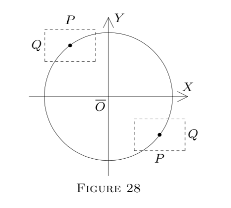
Por ejemplo, vamos

\[f(x, y)=x^{2}+y^{2}-25\]

(un polinomio; de ahí\(f \in C D^{1}\) en todo\(E^{2}).\) Geométricamente,\(x^{2}+y^{2}-25=0\) describe un círculo.

Resolviendo para\(x,\) obtenemos\(x=\pm \sqrt{25-y^{2}}.\) Así tenemos dos funciones:

\[H_{1}(y)=+\sqrt{25-y^{2}}\]

y

\[H_{2}(y)=-\sqrt{25-y^{2}}.\]

Si\(P \times Q\) está en la parte superior del círculo, la función resultante es\(H_{1}.\) De lo contrario, es\(H_{2}.\) Ver Figura 28.

V. Diferenciación implícita. El teorema 4 sólo afirma la existencia (y singularidad) de una solución, pero no muestra cómo encontrarla, en general.

El conocimiento mismo que\(H \in C D^{1}\) existe, sin embargo, nos permite utilizar su derivado o parciales y calcularlo por diferenciación implícita, conocida a partir del cálculo.

Ejemplos

a) Que\(f(x, y)=x^{2}+y^{2}-25=0,\) lo anterior.

Esta vez tratando\(y\) como una función implícita de\(x, y=H(x),\) y escribiendo\(y^{\prime}\) para\(H^{\prime}(x),\) diferenciamos ambos lados de (x^ {2} +y^ {2} -25=0\) con respecto al\(x,\) uso de la regla de cadena para el término\(y^{2}=[H(x)]^{2}\).

Esto rinde\(2 x+2 y y^{\prime}=0,\) de donde\(y^{\prime}=-x / y\).

En realidad (ver Nota 4), están involucradas dos funciones:\(y=\pm \sqrt{25-x^{2}};\) pero ambas satisfacen\(x^{2}+y^{2}-25=0;\) por lo que el resultado\(y^{\prime}=-x / y\) se aplica a ambas.

Por supuesto, este método sólo es posible si\(y^{\prime}\) se sabe que la derivada existe. Es por ello que el Teorema 4 es importante.

b) Dejar

\[f(x, y, z)=x^{2}+y^{2}+z^{2}-1=0, \quad x, y, z \in E^{1}.\]

De nuevo\(f\) satisface Teorema 4 para adecuado\(x, y,\) y\(z\).

Ajuste\(z=H(x, y),\) diferenciar la ecuación\(f(x, y, z)=0\) parcialmente con respecto a\(x\) y A\(y.\) partir de las dos ecuaciones resultantes, obtener\(\frac{\partial z}{\partial x}\) y\(\frac{\partial z}{\partial y}\).