1.2: Los ángulos y el producto de puntos

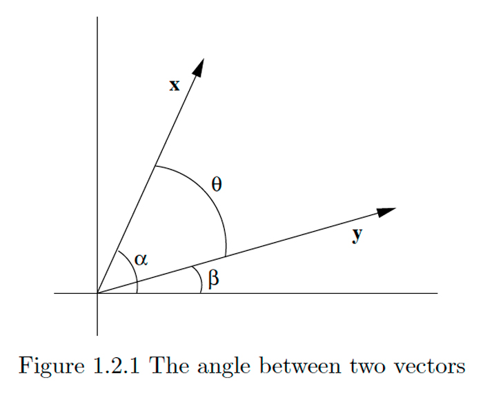
Supongamos\(\mathbf{x}=\left(x_{1}, x_{2}\right)\) y\(\mathbf{y}=\left(y_{1}, y_{2}\right)\) son dos vectores en\(\mathbf{R}^{2},\) ninguno de los cuales es el vector cero\(\mathbf{0}\). Dejar\(\alpha\) y\(\beta\) ser los ángulos entre\(\mathbf{x}\) y\(\mathbf{y}\) y el eje horizontal positivo, respectivamente, medidos en sentido contrario a las agujas del reloj. \(\alpha \geq \beta,\)Supongamos que\(\theta=\alpha-\beta\). Entonces\(\theta\) es el ángulo entre\(\mathbf{x}\) y\(\mathbf{y}\) medido en sentido contrario a las agujas del reloj, como se muestra en la Figura\(1.2 .1 .\) De la fórmula de resta para coseno tenemos

\[\cos (\theta)=\cos (\alpha-\beta)=\cos (\alpha) \cos (\beta)+\sin (\alpha) \sin (\beta).\]

Ahora

\[\cos (\alpha)=\frac{x_{1}}{\|x\|},\]

\[\cos (\beta)=\frac{y_{1}}{\|\mathbf{y}\|},\]

\[\sin (\alpha)=\frac{x_{2}}{\|\mathbf{x}\|},\]

y

\[ \sin(\beta)=\frac{y_2}{\|\mathbf{y}\|}.\]

Por lo tanto, tenemos

\[\cos (\theta)=\frac{x_{1} y_{1}}{\|x\|\|y\|}+\frac{x_{2} y_{2}}{\|x\|\|y\|}=\frac{x_{1} y_{1}+x_{2} y_{2}}{\|x\|\|y\|}.\]

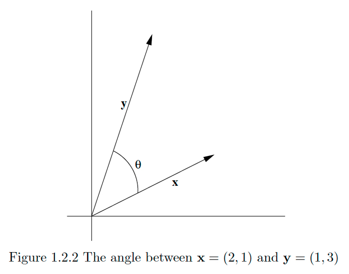
Ejemplo\(\PageIndex{1}\)

Dejar\(\theta\) ser el ángulo más pequeño entre\(\mathbf{x}=(2,1)\) y\(\mathbf{y}=(1,3),\) medido en el sentido contrario a las agujas del reloj. Entonces, por\((1.2 .2),\) debemos tener

\[\cos (\theta)=\frac{(2)(1)+(1)(3)}{\|\mathbf{x}\|\|\mathbf{y}\|}=\frac{5}{\sqrt{5} \sqrt{10}}=\frac{1}{\sqrt{2}}.\]

De ahí

\[\theta=\cos ^{-1}\left(\frac{1}{\sqrt{2}}\right)=\frac{\pi}{4}.\]

Ver Figura\(1.2 .2 .\)

Con más trabajo es posible demostrar que si\(\mathbf{x}=\left(x_{1}, x_{2}, x_{3}\right)\) y\(\mathbf{y}=\left(y_{1}, y_{2}, y_{3}\right)\) son dos vectores en\(\mathrm{R}^{3},\) ninguno de los cuales es el vector cero\(\mathbb{0},\) y\(\theta\) es el ángulo positivo más pequeño entre\(x\) y\(y,\) entonces

\[\cos (\theta)=\frac{x_{1} y_{1}+x_{2} y_{2}+x_{3} y_{3}}{\|\mathbf{x}\|\|\mathbf{y}\|}\]

El término que aparece en los numeradores en ambos\((1.2 .2)\) y\((1.2 .3)\) surge frecuentemente, por lo que le daremos un nombre.

Definición

Si\(\mathbf{x}=\left(x_{1}, x_{2}, \ldots, x_{n}\right)\) y\(\mathbf{y}=\left(y_{1}, y_{2}, \ldots, y_{n}\right)\) son vectores en\(\mathbb{R}^{n},\) entonces el producto de punto de\(\mathbf{x}\) y\(\mathbf{y},\) denotado\(\mathbf{x} \cdot \mathbf{y},\) viene dado por

\[\mathbf{x} \cdot \mathbf{y}=x_{1} y_{1}+x_{2} y_{2}+\cdots+x_{n} y_{n}.\]

Tenga en cuenta que el producto punto de dos vectores es un escalar, no otro vector. Debido a esto, el producto punto también se llama el producto escalar. También es un ejemplo de lo que se llama un producto interno y a menudo se denota por\(\langle\mathbf{x}, \mathbf{y}\rangle\).

Ejemplo\(\PageIndex{2}\)

Si\(x=(1,2,-3,-2)\) y\(y=(-1,2,3,5),\) entonces

\[\mathbf{x} \cdot \mathbf{y}=(1)(-1)+(2)(2)+(-3)(3)+(-2)(5)=-1+4-9-10=-16.\]

La siguiente proposición enumera algunas propiedades útiles del producto punto.

proposición\(\PageIndex{1}\)

Para cualquier vector\(\mathbf{x}, \mathbf{y},\) y\(\mathbf{z}\) en\(\mathbb{R}^{n}\) y escalar\(\boldsymbol{\alpha}\),

\[\mathbf{x} \cdot \mathbf{y}=\mathbf{y} \cdot \mathbf{x},\]

\[\mathbf{x} \cdot(\mathbf{y}+\mathbf{z})=\mathbf{x} \cdot \mathbf{y}+\mathbf{x} \cdot \mathbf{z},\]

\[(\alpha \mathbf{x}) \cdot \mathbf{y}=\alpha(\mathbf{x} \cdot \mathbf{y}),\]

\[0 \cdot \mathbb{x}=0,\]

\[\mathbf{x} \cdot \mathbf{x} \geq 0,\]

\[\mathbf{x} \cdot \mathbf{x}=0 \text { only if } \mathbf{x}=\mathbf{0},\]

y

\[\mathbf{x} \cdot \mathbf{x}=\|\mathbf{x}\|^{2}.\]

Todas estas propiedades son fácilmente verificables utilizando las propiedades de los números reales y la definición del producto punto y se dejarán al Problema 9 para que las verifiques.

En este punto podemos decir que si\(x\) y\(y\) son dos vectores distintos de cero en cualquiera\(\mathbb{R}^{2}\) o\(\mathbb{R}^{3}\) y\(\theta\) es el ángulo positivo más pequeño entre\(\mathbf{x}\) y\(\mathbf{y},\) entonces

\[\cos (\theta)=\frac{\mathbf{x} \cdot \mathbf{y}}{\|\mathbf{x}\|\|\mathbf{y}\|}.\]

Nos gustaría poder hacer la misma afirmación sobre el ángulo entre dos vectores en cualquier dimensión, pero primero tendríamos que definir a qué nos referimos con el ángulo entre dos vectores en\(\mathrm{R}^{n}\) for\(n>3 .\) La forma más sencilla de hacerlo es dar la vuelta a las cosas y usar\((1.2 .12)\) para definir el ángulo. Sin embargo, para que esto funcione primero debemos saber que
\[-1 \leq \frac{\mathbf{x} \cdot \mathbf{y}}{\|\mathbf{x}\|\|\mathbf{y}\|} \leq 1,\]
ya que este es el rango de valores para la función coseno. Este hecho se desprende de la siguiente desigualdad.

Desigualdad de Cauchy-Schwarz

Para todos\(x\) y\(y\) en\(\mathbb{R}^{n}\),
\[|\mathbf{x} \cdot \mathbf{y}| \leq\|\mathbf{x}\|\|\mathbf{y}\|.\]
Para ver por qué esto es así, primero tenga en cuenta que ambos lados de\((1.2 .13)\) son 0 cuando\(y=0,\) y por lo tanto son iguales en este caso. Asumiendo\(\mathrm{x}\) y\(\mathrm{y}\) son vectores fijos en\(\mathbb{R}^{n},\) con\(\mathrm{y} \neq 0,\) let\(t\) ser un número real y considerar la función
\[f(t)=(\mathbf{x}+t \mathbf{y}) \cdot(\mathbf{x}+t \mathbf{y}).\]
By\((1.2 .9), f(t) \geq 0\) para todo\(t,\) mientras desde\((1.2 .6),(1.2 .7),\) y\((1.2 .11),\) vemos que
\[f(t)=\mathbf{x} \cdot \mathbf{x}+\mathbf{x} \cdot t \mathbf{y}+t \mathbf{y} \cdot \mathbf{x}+t \mathbf{y} \cdot t \mathbf{y}=\|\mathbf{x}\|^{2}+2(\mathbf{x} \cdot \mathbf{y}) t+\|\mathbf{y}\|^{2} t^{2}.\]
De ahí\(f\) que sea un polinomio cuadrático con como máximo una raíz. Ya que las raíces de\(f\) son, como lo da la fórmula cuadrática,
\[\frac{-2(\mathbf{x} \cdot \mathbf{y}) \pm \sqrt{4(\mathbf{x} \cdot \mathbf{y})^{2}-4\|\mathbf{x}\|^{2}\|\mathbf{y}\|^{2}}}{2\|\mathbf{y}\|^{2}},\]
se deduce que debemos tener
\[4(\mathbf{x} \cdot \mathbf{y})^{2}-4\|\mathbf{x}\|^{2}\|\mathbf{y}\|^{2} \leq 0.\]
Así
\[(\mathbf{x} \cdot \mathbf{y})^{2} \leq\|\mathbf{x}\|^{2}\|\mathbf{y}\|^{2},\]
y así
\[|\mathbf{x} \cdot \mathbf{y}| \leq\|\mathbf{x}\|\|\mathbf{y}\|.\]
Tenga en cuenta que \(|\mathbf{x} \cdot \mathbf{y}|=\|\mathbf{x}\|\|\mathbf{y}\|\)si y solo si hay algún valor\(t\) para el\(f(t)=0,\) cual, por\((1.2 .8)\) y\((1.2 .10),\) sucede si y solo si\(x+t y=0,\) eso es,\(x=-t y,\) para algún valor de\(t .\) Por otra parte, si\(\mathbf{y}=\mathbf{0},\) entonces\(\mathbf{y}=0\mathbf{x}\), para alguno\(\mathbf{x}\) en\(\mathbb{R}^{n} .\) Por lo tanto, en cualquiera caso, la desigualdad Cauchy-Schwarz se convierte en una igualdad si y solo si cualquiera\(\mathbf{x}\) es un múltiplo escalar de\(\mathbf{y}\) o\(\mathbf{y}\) es un múltiplo escalar de\(\mathbf{x}\).
Con la desigualdad Cauchy-Schwarz tenemos
\[-1 \leq \frac{\mathbf{x} \cdot \mathbf{y}}{\|\mathbf{x}\|\|\mathbf{y}\|} \leq 1\]
para cualquier vector distinto de cero\(\mathbf{x}\) y\(\mathbf{y}\) en\(\mathbb{R}^{n} .\) Así podemos ahora exponer la siguiente definición.

Definición

Si\(x\) y\(y\) son vectores distintos de cero en\(\mathbb{R}^{n},\) entonces llamamos
\[\theta=\cos ^{-1}\left(\frac{\mathbf{x} \cdot \mathbf{y}}{\|\mathbf{x}\|\|\mathbf{y}\|}\right)\]
al ángulo entre\(\mathbf{x}\) y\(\mathbf{y} .\)

Ejemplo\(\PageIndex{3}\)

Supongamos\(\mathbf{x}=(1,2,3)\) y\(\mathbf{y}=(1,-2,2) .\) Entonces\(\mathbf{x} \cdot \mathbf{y}=1-4+6=3,\|\mathbf{x}\|=\sqrt{14}\), y\(\|\mathbf{y}\|=3,\) así si\(\theta\) es el ángulo entre\(\mathbf{x}\) y\(\mathbf{y},\) tenemos
\[\cos (\theta)=\frac{3}{3 \sqrt{14}}=\frac{1}{\sqrt{14}}.\]
Por lo tanto, redondeando a cuatro decimales,
\[\theta=\cos ^{-1}\left(\frac{1}{\sqrt{14}}\right)=1.3002.\]

Ejemplo\(\PageIndex{4}\)

Supongamos\(\mathbf{x}=(2,-1,3,1)\) y\(\mathbf{y}=(-2,3,1,-4) .\)\(\|\mathbf{y}\|=\sqrt{30},\) Entonces\(\mathbf{x} \cdot \mathbf{y}=-8,\|\mathbf{x}\|=\sqrt{15}\), y así si\(\theta\) es el ángulo entre\(\mathbf{x}\) y\(\mathbf{y},\) tenemos, redondeando a cuatro decimales,
\[\theta=\cos ^{-1}\left(\frac{-8}{\sqrt{15} \sqrt{30}}\right)=1.9575.\]

Ejemplo\(\PageIndex{5}\)

Dejar\(x\) ser un vector adentro\(\mathbb{R}^{n}\) y dejar\(\alpha_{k}, k=1,2, \ldots, n,\) ser el ángulo entre\(x\) y el eje\(k\) th. Entonces\(\alpha_{k}\) es el ángulo entre\(\mathbf{x}\) y el vector base estándar\(\mathbf{e}_{k} .\) Así es
\[\cos \left(\alpha_{k}\right)=\frac{\mathbf{x} \cdot \mathbf{e}_{k}}{\|\mathbf{x}\|\left\|\mathbf{e}_{k}\right\|}=\frac{x_{k}}{\|\mathbf{x}\|}.\]
decir,\(\cos \left(\alpha_{1}\right), \cos \left(\alpha_{2}\right), \ldots, \cos \left(\alpha_{n}\right)\) son los cosenos de dirección de\(\mathbf{x}\) como se define en la Sección 1.1. Por ejemplo, si\(\mathbf{x}=(3,1,2)\) en\(\mathbb{R}^{3},\) entonces\(\|\mathbf{x}\|=\sqrt{14}\) y la dirección cosenos de\(\mathbf{x}\) son
\[\begin{array}{l} {\cos \left(\alpha_{1}\right)=\frac{3}{\sqrt{14}}}, \\ {\cos \left(\alpha_{2}\right)=\frac{1}{\sqrt{14}}}, \end{array} \]
y
\[\cos \left(\alpha_{3}\right)=\frac{2}{\sqrt{14}},\]
dándonos, a cuatro decimales,
\[\begin{array}{l} {\alpha_{1}=0.6405} \\ {\alpha_{2}=1.3002} \end{array}\]
y
\[\alpha_{3}=1.0069\]
Tenga en cuenta que si\(x\) y\(y\) son vectores distintos de cero en\(\mathbb{R}^{n}\) con\(x \cdot y=0,\) entonces el ángulo entre x e y es
\[\cos ^{-1}(0)=\frac{\pi}{2}.\]
Esta es la motivación detrás de nuestra siguiente definición.

Definición

Se dice que\(\mathbb{R}^{n}\) los vectores\(\mathrm{x}\) y\(\mathrm{y}\) en son ortogonales (o perpendiculares), denotados\(\mathbf{x} \perp \mathbf{y},\) si\(\mathbf{x} \cdot \mathbf{y}=0\).

Es una convención conveniente de las matemáticas para no restringir la definición de ortogonalidad a vectores distintos de cero. De ahí se desprende de la definición, y\((1.2 .8),\) que 0 es ortogonal a cada vector en\(\mathbb{R}^{n} .\) Además, 0 es el único vector en el\(\mathbb{R}^{n}\) que tiene esta propiedad, hecho que se le pedirá que verifique en el Problema 12.

Ejemplo\(\PageIndex{6}\)

Los vectores\(\mathbf{x}=(-1,-2)\) y\(\mathbf{y}=(1,2)\) son ambos ortogonales a\(\mathbf{z}=(2,-1)\) en\(\mathbb{R}^{2} .\) Note que\(\mathbf{y}=-\mathbf{x}\) y, de hecho, cualquier múltiplo escalar de\(\mathbf{x}\) es ortogonal a z.

Ejemplo\(\PageIndex{7}\)

En\(\mathbb{R}^{4}, \mathbf{x}=(1,-1,1,-1)\) es ortogonal a\(\mathbf{y}=(1,1,1,1) .\) Como en el ejemplo anterior, cualquier múltiplo escalar de\(\mathbf{x}\) es ortogonal a\(\mathbf{y}\).

Definición

Decimos vectores\(\mathbf{x}\) y\(\mathbf{y}\) son paralelos si\(\mathbf{x}=\alpha \mathbf{y}\) para algún escalar\(\alpha \neq 0\).

Esta definición dice que los vectores son paralelos cuando uno es un múltiplo escalar distinto de cero del otro. De nuestra prueba de la desigualdad Cauchy-Schwarz sabemos que se deduce que si\(x\) y\(y\) son paralelos, entonces\(|x \cdot y|=\|x\| \| y | .\) así si\(\theta\) es el ángulo entre\(x\) y\(y\), Es
\[\cos (\theta)=\frac{\mathbf{x} \cdot \mathbf{y}}{\|\mathbf{x}\|\|\mathbf{y}\|}=\pm 1.\]
decir,\(\theta=0\) o\(\theta=\pi .\) Dicho de otra manera, \(x\)y\(y\) bien apuntan en la misma dirección o apuntan en direcciones opuestas.

Ejemplo\(\PageIndex{8}\)

Los vectores\(x=(1,-3)\) y\(y=(-2,6)\) son paralelos desde\(x=-\frac{1}{2} y .\) Tenga en cuenta que\(\mathbf{x} \cdot \mathbf{y}=-20\) y\(\|\mathbf{x}\|\|\mathbf{y}\|=\sqrt{10} \sqrt{40}=20,\) así\(\mathbf{x} \cdot \mathbf{y}=-\|\mathbf{x}\|\|\mathbf{y}\| .\) Se deduce que el ángulo entre\(x\) y\(y\) es\(\pi\).

Dos resultados básicos sobre triángulos en\(\mathbb{R}^{2}\) y\(\mathbb{R}^{3}\) son la desigualdad del triángulo (la suma de las longitudes de dos lados de un triángulo es mayor o igual a la longitud del tercer lado\()\) y el teorema de Pitágoras (la suma de los cuadrados de las longitudes de las patas de un triángulo rectángulo es igual al cuadrado de la longitud del otro lado). En términos de vectores en\(\mathbb{R}^{n},\) si nos imagino un vector\(\mathbf{x}\) con su cola en el origen y un vector\(\mathbf{y}\) con su cola en la punta de\(\mathbf{x}\) como dos lados de un triángulo, entonces el lado restante viene dado por el vector\(\mathbf{x}+\mathbf{y}\). Así, la desigualdad triangular se puede afirmar de la siguiente manera.

Desigualdad triangular

Si\(x\) y\(y\) son vectores en\(\mathbb{R}^{n},\) entonces
\[\|\mathbf{x}+\mathbf{y}\| \leq\|\mathbf{x}\|+\|\mathbf{y}\|.\]
El primer paso para verificar\((1.2 .21)\) es señalar que, usando\((1.2 .11)\) y\((1.2 .6)\),
\[ \begin{aligned} \|\mathbf{x}+\mathbf{y}\|^{2} &=(\mathbf{x}+\mathbf{y}) \cdot(\mathbf{x}+\mathbf{y}) \\ &=\mathbf{x} \cdot \mathbf{x}+2(\mathbf{x} \cdot \mathbf{y})+\mathbf{y} \cdot \mathbf{y} \\ &=\|\mathbf{x}\|^{2}+2(\mathbf{x} \cdot \mathbf{y})+\|\mathbf{y}\|^{2} \end{aligned}\]
Desde\(\mathbf{x} \cdot \mathbf{y} \leq\|\mathbf{x}\|\|\mathbf{y}\|\) por la desigualdad Cauchy-Schwarz, se deduce que
\[\|\mathbf{x}+\mathbf{y}\|^{2} \leq \| \mathbf{x}\left\|^{2}+2\right\| \mathbf{x}\|\| \mathbf{y}\|+\| \mathbf{y}\left\|^{2}=(\|\mathbf{x}\|+\|\mathbf{y}\|)^{2}\right.\]
de donde obtenemos la desigualdad triangular tomando raíces cuadradas.
Tenga en cuenta que en\((1.2 .22)\) tenemos
\[\|\mathbf{x}+\mathbf{y}\|^{2}=\|\mathbf{x}\|^{2}+\|\mathbf{y}\|^{2}\]
si y solo si\(x \cdot y=0,\) eso es, si y solo si\(x \perp y .\) De ahí tenemos el siguiente resultado famoso.

Teorema de Pitágoras

Los vectores\(\mathbf{x}\) y\(\mathbf{y}\) en\(\mathbb{R}^{n}\) son ortogonales si y solo si
\[\|\mathbf{x}+\mathbf{y}\|^{2}=\|\mathbf{x}\|^{2}+\|\mathbf{y}\|^{2}.\]

Quizás la aplicación más importante del producto punto es encontrar la proyección ortogonal de un vector sobre otro. Esto se ilustra en la Figura\(1.2 .3,\) donde w representa la proyección de\(x\) sobre\(y .\) El resultado de la proyección es romper\(x\) en la suma de dos componentes,\ mathbf {w}, que es paralelo a\(\mathbf{y},\) y\(\mathbf{x}-\mathbf{w},\) que es ortogonal a\(\mathbf{y},\) un procedimiento que es frecuentemente muy útil. Para calcular\ mathbf {w}, tenga en cuenta que si\(\theta\) es el ángulo entre\(\mathbf{x}\) y\(\mathbf{y},\) entonces
\[\|\mathbf{w}\|=\|\mathbf{x}\|\left|\cos (\theta)\left|=\|\mathbf{x}\| \frac{|\mathbf{x} \cdot \mathbf{y}\|}{\|\mathbf{x}\|\|\mathbf{y}\|}=\right| \mathbf{x} \cdot \frac{\mathbf{y}}{\|\mathbf{y}\|}\right|=| \mathbf{x} \cdot \mathbf{u} |,\]
donde
\[\mathbf{u}=\frac{\mathbf{y}}{\|\mathbf{y}\|}\]
esta la dirección de\(\mathbf{y} .\) Por lo tanto\(\mathbf{w}=|\mathbf{x} \cdot \mathbf{u}| \mathbf{u}\) cuando\(0 \leq \theta \leq \frac{\pi}{2},\) que es cuando\(\mathbf{x} \cdot \mathbf{u}>0,\) y
\(\mathbf{w}=-|\mathbf{x} \cdot \mathbf{u}| \mathbf{u}\)cuando\(\frac{\pi}{2}<\theta \leq \pi,\) que es cuando\(\mathbf{x} \cdot \mathbf{u}<0 .\) Así, en cualquier caso,\(\mathbf{w}=(\mathbf{x} \cdot \mathbf{u}) \mathbf{u}\).

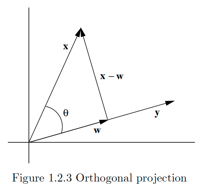
Definición

Dados vectores\(\mathbf{x}\) y\(\mathbf{y}, \mathbf{y} \neq \mathbf{0},\) en\(\mathbb{R}^{n},\) el vector
\[\mathbf{w}=(\mathbf{x} \cdot \mathbf{u}) \mathbf{u},\]
donde\(\mathbf{u}\) está la dirección de\(\mathbf{y},\) se llama la proyección ortogonal, o simplemente proyección, de\(\mathbf{x}\) sobre y También llamamos w el componente de\(x\) en la dirección de \(y\)y\(x \cdot u\) la coordenada de\(x\) en la dirección de\(y .\)

En el caso especial donde\(\mathrm{y}=\mathbf{e}_{k},\) el\(k\) th vector básico estándar,\(k=1,2, \ldots, n,\) vemos que la coordenada de\(\mathbf{x}=\left(x_{1}, x_{2}, \ldots, x_{n}\right)\) en la dirección de\(y\) es solo\(x \cdot e_{k}=x_{k},\) la coordenada\(k\) th de\(\mathbf{x}\).

Ejemplo\(\PageIndex{9}\)

Supongamos\(\mathbf{x}=(1,2,3)\) y\(\mathbf{y}=(1,4,0) .\) Entonces la dirección de\(\mathbf{y}\) es
\[\mathbf{u}=\frac{1}{\sqrt{17}}(1,4,0),\]
así la coordenada de\(x\) en la dirección de\(y\) es
\[\mathbf{x} \cdot \mathbf{u}=\frac{1}{\sqrt{17}}(1+8+0)=\frac{9}{\sqrt{17}}.\]
Así la proyección de\(x\) sobre\(y\) es
\[\mathbf{w}=\frac{9}{\sqrt{17}} \mathbf{u}=\frac{9}{17}(1,4,0)=\left(\frac{9}{17}, \frac{36}{17}, 0\right).\]