1.3: El Producto Cruzado

Como señalamos en la Sección 1.1, no existe una manera general de definir la multiplicación para vectores en\(\mathbb{R}^{n}\), siendo el producto también un vector de la misma dimensión, lo cual es útil para nuestros propósitos en este libro. No obstante, en el caso especial de que\(\mathbb{R}^{3}\) haya un producto que nos resultará útil. Una motivación para este producto es considerar el siguiente problema: Dados dos vectores\(\mathbf{x}=\left(x_{1}, x_{2}, x_{3}\right)\) y\(\mathbf{y}=\left(y_{1}, y_{2}, y_{3}\right)\) en\(\mathbb{R}^{3}\), no paralelos entre sí, encontrar un tercer vector\(\mathbf{w}=\left(w_{1}, w_{2}, w_{3}\right)\) que es ortogonal a ambos\(\mathbf{x}\) y\(\mathbf{y}\). Así queremos\(\mathbf{w} \cdot \mathbf{x}=0\) y\(\mathbf{w} \cdot \mathbf{y}=0\), lo que significa que necesitamos resolver las ecuaciones

\[x_1w_1 + x_2w_2+x_3w_3=0 \\ y_1w_1 + y_2w_2+y_3w_3=0 \label{1.3.1}\]

para\(w_1\),\(w_2\), y\(w_3\). Multiplicar la primera ecuación por\(y_3\) y la segunda por nos\(x_3\) da

\[x_1y_3w_1 + x_2y_3w_2 + x_3y_3w_3 = 0 \\ x_3y_1w_1 + x_3y_2w_2 + x_3y_3w_3 = 0 . \label{1.3.2} \]

Restando la segunda ecuación de la primera, tenemos

\[ (x_1y_3-x_3y_1)w_1 + (x_2y_3-x_3y_2)w_2=0 . \label{1.3.3}\]

Una solución de Ecuación\ ref {1.3.3} viene dada por la configuración

\[w_1=x_2y_3-x_3y_2 \\ w_2=-(x_1y_3-x_3y_1) = x_3y_1-x_1y_3 . \label{1.3.4}\]

Finalmente, a partir de la primera ecuación en la Ecuación\ ref {1.3.1}, ahora tenemos

\[x_3w_3=-x_1(x_2y_3-x_3y_2)-x_2(x_3y_1-x_1y_3)=x_1x_3y_2-x_2x_3y_1 , \label{1.3.5}\]

de la que obtenemos la solución

\[w_3=x_1y_2-x_2y_1 . \label{1.3.6}\]

Las elecciones hechas al llegar a la Ecuación\ ref {1.3.4} y\ ref {1.3.6} no son únicas, sino que son las elecciones estándar que definen\(\mathbf{w}\) como el producto cruzado o vectorial de\(\mathbf{x}\) y\(\mathbf{y}\).

Definición\(\PageIndex{1}\)

Vectores dados\(\mathbf{x}=\left(x_{1}, x_{2}, x_{3}\right)\) y\(\mathbf{y}=\left(y_{1}, y_{2}, y_{3}\right)\) en\(\mathbb{R}^{3}\), el vector

\[ \mathbf{x}\times \mathbf{y}=(x_2y_3-x_3y_2,x_3y_1-x_1y_3,x_1y_2-x_2y_1)\]

se llama el producto cruzado, o producto vectorial, de\(\mathbf{x}\) y\(\mathbf{y}\).

Ejemplo\(\PageIndex{1}\)

Si\(\mathbf{x}=(1,2,3)\) y\(\mathbf{y}=(1,-1,1)\), entonces

\[\mathbf{x} \times \mathbf{y} = (2 + 3,3 − 1,−1 − 2) = (5,2,−3) . \nonumber \]

Tenga en cuenta que

\[\mathbf{x} \cdot (\mathbf{x} \times \mathbf{y}) = 5+4-9=0 \nonumber\]

y

\[\mathbf{y} \cdot (\mathbf{x} \times \mathbf{y})=5-2-3=0 , \nonumber \]

demostrando eso\(\mathbf{x} \perp (\mathbf{x} \times \mathbf{y})\) y\( \mathbf{y} \perp (\mathbf{x} \times \mathbf{y}) \) como se afirma. También es interesante señalar que

\[\mathbf{y}\times \mathbf{x}=(-3-2,1-3,2+1)=(-5,-2,3)=-(\mathbf{x}\times \mathbf{y}) . \nonumber\]

Este último cálculo se mantiene en general para todos los vectores\(\mathbf{x}\) y\(\mathbf{y}\) en\(\mathbb{R}^{3}\).

Proposición\(\PageIndex{1}\)

Supongamos\(\mathbf{x}\)\(\mathbf{y}\),, y\(\mathbf{z}\) son vectores en\(\mathbb{R}^3\) y\(\alpha\) es cualquier número real. Entonces

\[\mathbf{x}\times \mathbf{y} = -(\mathbf{y} \times \mathbf{x}) , \]

\[\mathbf{x} \times (\mathbf{y}+\mathbf{z}) = (\mathbf{x} \times \mathbf{y}) + (\mathbf{x} \times \mathbf{z}) , \]

\[(\mathbf{x}+\mathbf{y}) \times \mathbf{z} = (\mathbf{x} \times \mathbf{z}) + (\mathbf{y} \times \mathbf{z}) , \]

\[ \alpha (\mathbf{x} \times \mathbf{y}) = (\alpha \mathbf{x}) \times \mathbf{y} = \mathbf{x} \times (\alpha \mathbf{y}) , \]

y

\[\mathbf{x} \times \mathbf{0} = \mathbf{0} . \]

La verificación de estas propiedades es sencilla y se dejará al Ejercicio 10. Además, observe que

\[\mathbf{e}_1 \times \mathbf{e}_2 = \mathbf{e}_3 , \]

\[\mathbf{e}_2 \times \mathbf{e}_3 = \mathbf{e}_1 , \]

y

\[\mathbf{e}_3 \times \mathbf{e}_1 = \mathbf{e}_2 ; \]

es decir, el producto cruzado de dos vectores base estándar es el otro vector base estándar o su negativo. Además, tenga en cuenta que en estos casos el producto cruzado apunta en la dirección que apuntaría tu pulgar si envolvieras los dedos de tu mano derecha del primer vector al segundo. Esto de hecho siempre es cierto y da como resultado lo que se conoce como regla de la mano derecha para la orientación del producto cruzado, como se muestra en la Figura 1.3.1. De ahí dados dos vectores\(\mathbf{x}\) y\(\mathbf{y}\), siempre podemos determinar la dirección de\(\mathbf{x} \times \mathbf{y}\); a

Figura\(\PageIndex{1}\): La regla de la derecha

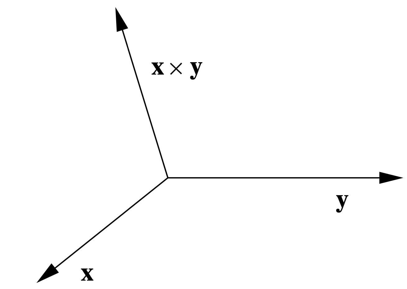
identificar completamente\(\mathbf{x} \times \mathbf{y}\) geométricamente, sólo necesitamos conocer su longitud. Ahora bien, si θ es el ángulo entre\(\mathbf{x}\) y\(\mathbf{y}\), entonces

\ begin {align}
\ |\ mathbf {x}\ times\ mathbf {y}\ |^ {2} =&\ left (x_ {2} y_ {3} -x_ {3} y_ {2}\ derecha) ^ {2} +\ izquierda (x_ {3} y_ {1} -x_ {1} y_ {3}\ derecha) ^ {2} +\ izquierda (x_ {1} y_ {2} -x_ {2} y_ {1}\ derecha) ^ {2}\ nonumber\\
=& x_ {2} ^ {2} y_ {3} ^ {2} -2 x_ {2} x_ {3} y_ {2} y_ {3} +x_ {3} ^ {2} y_ {2} ^ 2} +x_ {3} ^ {2} y_ {1} ^ {2} -2 x_ {1} x_ {3} y_ {1} y_ {3} +x_ {1} ^ {2} y_ {3} ^ {2} +x_ {1} ^ {2} y_ {2} ^ {2}\ nonumber\\
&\ quad-2 x_ {1} x_ {2} y_ {1} y_ {2} +x_ {2} +x_ {2}} ^ {2} y_ {1} ^ {2}\ nonumber\\
=&\ izquierda (x_ {1} ^ {2} +x_ {2} ^ {2} +x_ {3} ^ {2}\ derecha)\ izquierda (y_ {1} ^ {2} +y_ {2} ^ {2} +y_ {3} ^ {2}\ derecha) -\ izquierda (x_ {1} ^ {2} y_ {1} ^ {2} +x_ {2} ^ {2} y_ {2} ^ {2} +x_ {3} ^ {2} y_ {3} ^ {2}\ derecha)\ nonumber\\
&\ quad-\ izquierda (2 x_ {2} x_ {3} y_ {2} y_ {3} +2 x_ {1} x_ {3} y_ {1} y_ {3} +2 x_ {1} x_ {2} y_ {2} y_ {1} y_ {2}\ derecha)\ nonumber\\
=&\ izquierda (x_ {1} ^ {2} +x_ {2} ^ {2} +x_ {3} ^ {2}\ derecha)\ izquierda (y_ {1} ^ {2} +y_ {2} ^ {2} +y_ {3} ^ {2}\ derecha) -\ izquierda (x_ {1} y_ {1} +x_ {2} y_ {2} +x_ { 3} y_ {3}\ derecha) ^ {2}\ nonumber\\
=&\ |\ mathbf {x}\ |^ {2}\ |\ mathbf {y}\ |^ {2} - (\ mathbf {x}\ cdot\ mathbf {y}) ^ {2}\ nonumber\\
=&\ |\ mathbf {x}\ |^ {2}\ |\ mathbf {y}\ |^ {2} - (\ |\ mathbf {x}\ |\ |\ mathbf {y}\ |\ cos (\ theta)) ^ {2}\ nonumber\\
=&\ |\ mathbf {x}\ |^ {2}\ |\ mathbf {y}\ |^ {2 }\ izquierda (1-\ cos ^ {2} (\ theta)\ derecha)\ nonumber\\
=&\ |\ mathbf {x}\ |^ {2}\ |\ mathbf {y}\ |^ {2}\ sin ^ {2} (\ theta). \ label {}
\ end {align}

Tomando raíces cuadradas, y señalando que\(\sin(\theta) \geq 0 \) ya que, por la definición del ángulo entre dos vectores\(0 \leq \theta \leq \pi \),, tenemos el siguiente resultado.

Proposición\(\PageIndex{2}\)

Si θ es el ángulo entre dos vectores\(\mathbf{x}\) e\(\mathbf{y}\) in\(\mathbb{R}^{3}\), entonces

\[ \| \mathbf{x} \times \mathbf{y} \| = \| \mathbf{x} \| \| \mathbf{y} \| \sin (\theta) . \label{1.3.17} \]

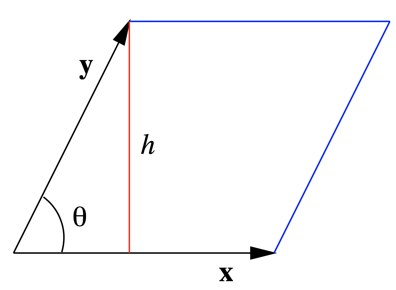
El último teorema tiene varias consecuencias interesantes. Uno de estos proviene de reconocer que si dibujamos un paralelogramo con\(\mathbf{x}\) y\(\mathbf{y}\) como lados adyacentes, como en la Figura 1.3.2, entonces la altura del paralelogramo es\(\| \mathbf{y} \| \sin(\theta)\), donde θ es el ángulo entre\(\mathbf{x}\) y\(\mathbf{y}\). De ahí que el área del paralelogramo sea\(\| \mathbf{x} \| \| \mathbf{y} \| \sin(\theta)\), que por Ecuación\ ref {1.3.17} es\(\| \mathbf{x} \times \mathbf{y} \|\).

Figura\(\PageIndex{2}\): La altura del paralelogramo es\(h=\| \mathbf{y} \| \sin(\theta)\)

Proposición\(\PageIndex{3}\)

Supongamos\(\mathbf{x}\) y\(\mathbf{y}\) son dos vectores en\(\mathbb{R}^{3}\). Entonces el área del paralelogramo que tiene\(\mathbf{x}\) y\(\mathbf{y}\) para lados adyacentes es\(\| \mathbf{x} \times \mathbf{y} \| \).

Ejemplo\(\PageIndex{2}\)

Considera el paralelogramo\(P\) con vértices en (0, 0, 0), (6, 1, 1), (8, 5, 2) y (2, 4, 1). Dos lados adyacentes son especificados por los vectores\(\mathbf{x}=(6,1,1)\) y\(\mathbf{y}=(2,4,1)\) (ver Figura 1.3.3), por lo que el área de\(P\) es

\[\| \mathbf{x} \times \mathbf{y} \| = \|(1-4,2-6,24-2) \| = \| (-3,-4,22 \| = \sqrt{509} . \nonumber \]

Ver Figura 1.3.4 para ver la relación entre\(\mathbf{x} \times \mathbf{y}\) y\(P\).

Figura\(\PageIndex{3}\): Paralelogramo con vértices en (0, 0, 0), (6, 1, 1), (8, 5, 2) y (2, 4, 1)

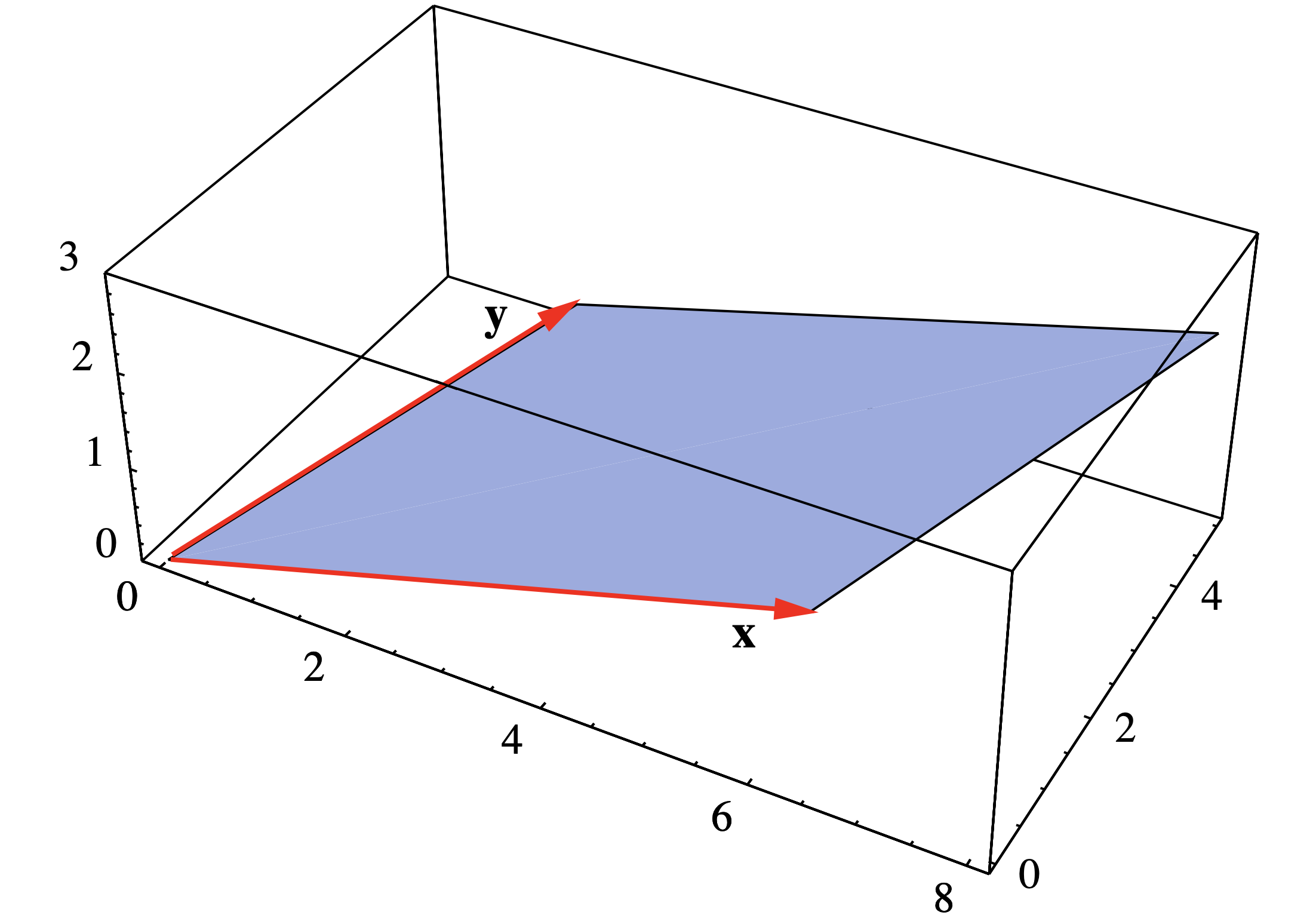
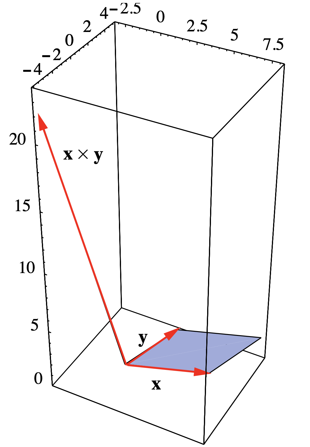
Figura 1.3.4 Paralelogramo con lados adyacentes\(\mathbf{x}=(6,1,1)\) y\(\mathbf{y}=(2,4,1)\)

Ejemplo\(\PageIndex{3}\)

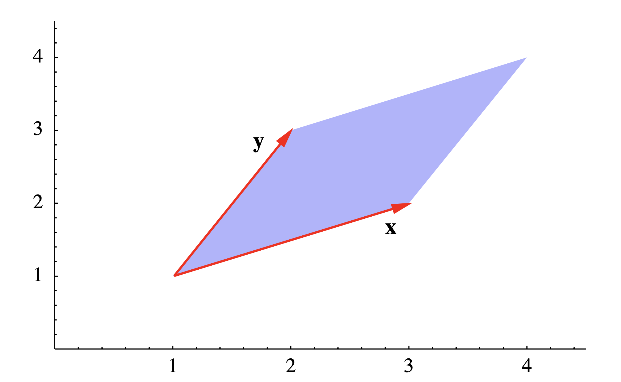
Considere el paralelogramo\(P\) en el plano con vértices en (1, 1,), (3, 2), (4, 4) y (2, 3). Dos lados adyacentes están dados por los vectores de (1, 1) a (3, 2), es decir

\[\mathbf{x} = (3,2) - (1,1) = (2,1) , \nonumber \]

y de (1,1) a (2,3), es decir,

\[\mathbf{y}=(2,3)-(1,1)=(1,2) . \nonumber\]

Ver Figura 1.3.5. Sin embargo, dado que estos vectores están en\(\mathbb{R}^2\), no en\(\mathbb{R}^3\), no podemos calcular su producto cruzado. Para sortear esto, consideramos los vectores\(\mathbf{w}=(2,1,0)\) y\(\mathbf{v}=(1,2,0)\) que son lados adyacentes del mismo paralelogramo vistos como tumbados en\(\mathbb{R}^3\). Entonces el área de\(P\) es dada por\[ \| \mathbf{w} × \mathbf{v} \| = \| (0,0,4 − 1) \| = \| (0,0,3)\| = 3 . \nonumber \]

Figura\(\PageIndex{5}\): Paralelogramo con vértices en (1, 1), (3, 2), (4, 4) y (2, 3)

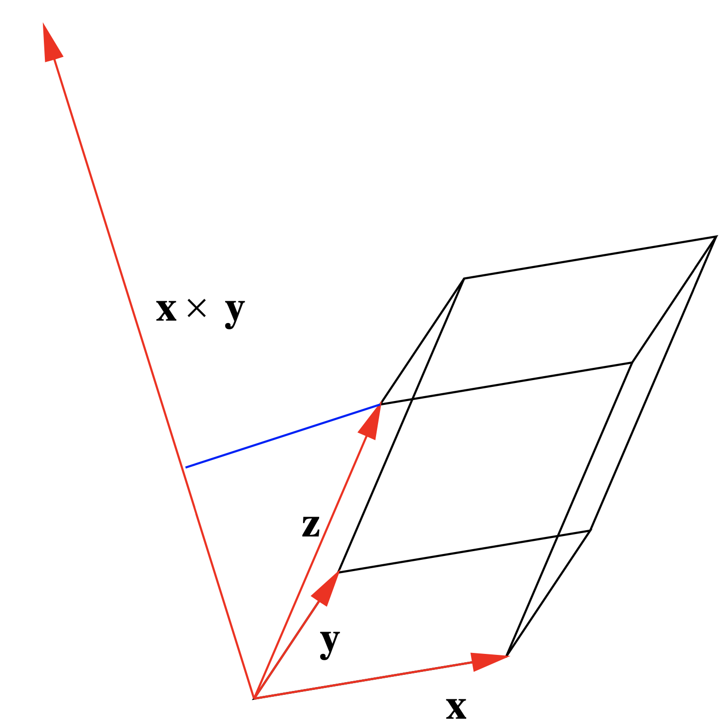
Es fácil extender el resultado del teorema anterior para computar el volumen de un paralelepípedo en\(\mathbb{R}^3\). Supongamos\(\mathbf{x}\)\(\mathbf{y}\),, y\(\mathbf{z}\) son bordes adyacentes de paralelepípedo\(P\), como se muestra en la Figura 1.3.6. Entonces el volumen\(V\) de\(P\) es\(\| \mathbf{x} \times \mathbf{y} \| \), que es el área de la base, multiplicado por la altura de\(P\), que es la longitud de la proyección de\(\mathbf{z}\) sobre\(\mathbf{x} \times \mathbf{y}\). Dado que este último es igual a

\[ \left| \mathbf{z} \cdot \frac{\mathbf{x} \times \mathbf{y}}{\| \mathbf{x} \times \mathbf{y} \|} \right| , \nonumber \]

Figura\(\PageIndex{6}\): Paralelepípedo con bordes adyacentes\(\mathbf{x}\),\(\mathbf{y}\), y\(\mathbf{z}\)

tenemos

\[V = \| \mathbf{x} \times \mathbf{y} \| \left| z \cdot \frac{\mathbf{x} \times \mathbf{y}}{\| \mathbf{x} \times \mathbf{y} \|} \right| = \vert \mathbf{z} \cdot (\mathbf{x} \times \mathbf{y}) \vert . \]

Proposición\(\PageIndex{4}\)

El volumen de un paralelepípedo con bordes adyacentes\(\mathbf{x}\),\(\mathbf{y}\), y\(\mathbf{z}\) es\( \vert \mathbf{z} \cdot (\mathbf{x} \times \mathbf{y}) \vert \).

Definición\(\PageIndex{2}\)

Dados tres vectores\(\mathbf{x}\)\(\mathbf{y}\),, y\(\mathbf{z}\) en\(\mathbb{R}^3\), la cantidad\( \mathbf{z} \cdot (\mathbf{x} \times \mathbf{y}) \) se llama el producto triple escalar de\(\mathbf{x}\),\(\mathbf{y}\), y\(\mathbf{x}\).

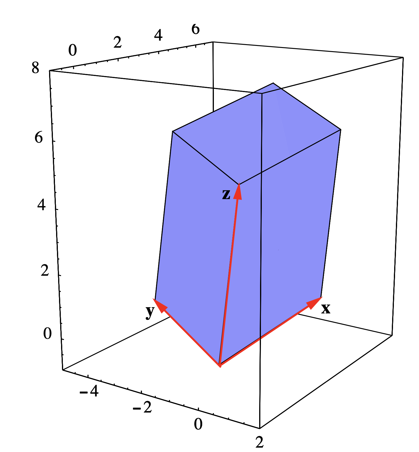
Ejemplo\(\PageIndex{4}\)

Dejar\(\mathbf{x}=(1,4,1)\),\(\mathbf{y}=(-3,1,1)\), y\(\mathbf{z}=(0,1,5)\) ser bordes adyacentes de paralelepípedo\(P\) (ver Figura 1.3.7). Entonces\[\mathbf{x} \times \mathbf{y} = (4-1,-3-1,1+12) = (3,-4,13) , \nonumber \]

por lo

\[\mathbf{z} \cdot (\mathbf{x} \times \mathbf{y}) = 0-4+65 = 61. \nonumber \]

De ahí que el volumen de\(P\) sea 61.

Figura\(\PageIndex{7}\): Paralelepípedo con bordes adyacentes\(\mathbf{x} = (1, 4, 1), \mathbf{y} = (−3, 1, 1), \mathbf{z} = (0, 1, 5)\)

El resultado final de esta sección se desprende de la Ecuación\ ref {1.3.17} y el hecho de que el ángulo entre vectores paralelos es 0 o\(\pi\).

Proposición\(\PageIndex{5}\)

Los vectores\(\mathbf{x}\) y\(\mathbf{y}\) en\(\mathbb{R}^3\) son paralelos si y solo si\(\mathbf{x} \times \mathbf{y}=\mathbf{0}\).

Tenga en cuenta que, en particular, para cualquier vector\(\mathbf{x}\) en\(\mathbb{R}^3\),\(\mathbf{x} \times \mathbf{x}=\mathbf{0}\).