1.5: Funciones lineales y afín

Uno de los temas centrales del cálculo es la aproximación de funciones no lineales por funciones lineales, siendo el concepto fundamental la derivada de una función. En esta sección se introducirán las funciones lineales y afines que serán claves para entender las derivadas en los capítulos venideros.

Funciones lineales

A continuación, usaremos la notación\( f: \mathbb{R}^{m} \rightarrow \mathbb{R}^{n} \) para indicar una función cuyo dominio es un subconjunto de\(\mathbb{R}^{m}\) y cuyo rango es un subconjunto de\( \mathbb{R}^{n}\). En otras palabras,\(f\) toma un vector con\(m\) coordenadas para la entrada y devuelve un vector con\(n\) coordenadas. Por ejemplo, la función

\[ f(x, y, z)=\left(\sin (x+y), 2 x^{2}+z\right) \nonumber \]

es una función de\( \mathbb{R}^{3}\) a\(\mathbb{R}^{2}\).

Definición\(\PageIndex{1}\)

Decimos que una función\(L: \mathbb{R}^{m} \rightarrow \mathbb{R}^{m}\) es lineal si (1) para cualquier vector\(\mathbf{x}\) y\(\mathbf{y}\) en\(\mathbb{R}^{m}\),

\[ L(\mathbf{x}+\mathbf{y})=L(\mathbf{x})+L(\mathbf{y}), \]

y (2) para cualquier vector\(\mathbf{x}\) en\(\mathbb{R}^{m}\) y escalar\(a\),

\[ L(a \mathbf{x})=a L(\mathbf{x}). \]

Ejemplo\(\PageIndex{1}\)

Supongamos que\(f: \mathbb{R} \rightarrow \mathbb{R}\) está definido por\(f(x)=3 x\). Entonces para cualquiera\(x\) y\(y\) en\(\mathbb{R}\),

\[ f(x+y)=3(x+y)=3 x+3 y=f(x)+f(y), \nonumber \]

y para cualquier escalar\(a\),

\[ f(a x)=3 a x=a f(x). \nonumber \]

Así\(f\) es lineal.

Ejemplo\(\PageIndex{2}\)

Supongamos que\(L: \mathbb{R}^{2} \rightarrow \mathbb{R}^{3}\) está definido por

\[ L\left(x_{1}, x_{2}\right)=\left(2 x_{1}+3 x_{2}, x_{1}-x_{2}, 4 x_{2}\right). \nonumber \]

Entonces si\(\mathbf{x}=\left(x_{1}, x_{2}\right)\) y\(\mathbf{y}=\left(y_{1}, y_{2}\right)\) son vectores en\(\mathbb{R}^2\),

\ [\ begin {alineado}
L (\ mathbf {x} +\ mathbf {y}) &=L\ izquierda (x_ {1} +y_ {1}, x_ {2} +y_ {2}\ derecha)\\
&=\ izquierda (2\ izquierda (x_ {1} +y_ {1}\ derecha) +3\ izquierda (x_ {2} +y_ {2} +y_ {2}}\ derecha), x_ {1} +y_ {1} -\ izquierda (x_ {2} +y_ {2}\ derecha), 4\ izquierda (x_ {2} +y_ {2}\ derecha)\ derecha)\\
&=\ izquierda (2 x_ {1} +3 x_ {2}, x_ {1} -x_ { 2}, 4 x_ {2}\ derecha) +\ izquierda (2 y_ {1} +3 y_ {2}, y_ {1} -y_ {2}, 4 y_ {2}\ derecha)\\
&=L\ izquierda (x_ {1}, x_ {2}\ derecha) +L\ izquierda (y_ {1}, y_ {2}\ derecha)\
&=L (\ mathbf {x}) +L (\ mathbf {y}).
\ end {alineado}\]

Además, para\( \mathbf{x}=\left(x_{1}, x_{2}\right)\) y cualquier escalar\(a\), tenemos

\ [\ begin {alineado}
L (a\ mathbf {x}) &=L\ izquierda (a x_ {1}, a x_ {2}\ derecha)\\
&=\ izquierda (2 a x_ {1} +3 a x_ {2}, a x_ {1} -a x_ {2}, 4 a x_ {2}\ derecha)\\
&=a\ izquierda (2 x_ _ {2} +3 x_ {2}, x_ {1} -x_ {2}, 4 x_ {2}\ derecha)\\
&=a L (\ mathbf {x}).
\ end {alineado}\]

Así\(L\) es lineal.

Ahora supongamos que\( L: \mathbb{R} \rightarrow \mathbb{R}\) es una función lineal y vamos\(a=L(1)\). Entonces para cualquier número real\(x\),

\[ L(x)=L(1 x)=x L(1)=a x. \]

Dado que cualquier función\(L: \mathbb{R} \rightarrow \mathbb{R}\) definida por\(L(x)=a x\), donde\(a\) es un escalar, es lineal (ver Ejercicio 1), se deduce que las únicas funciones\( L: \mathbb{R} \rightarrow \mathbb{R}\) que son lineales son las de la forma\(L(x)=a x\) para algún número real\(a\). Por ejemplo,\(f(x)=5 x\) es una función lineal, pero no\(g(x)=\sin (x) \) lo es.

A continuación, supongamos que\(L: \mathbb{R}^{m} \rightarrow \mathbb{R}\) es lineal y vamos\(a_{1}=L\left(\mathbf{e}_{1}\right), a_{2}=L\left(\mathbf{e}_{2}\right), \ldots, a_{m}=L\left(\mathbf{e}_{m}\right)\). Si\(\mathbf{x}=\left(x_{1}, x_{2}, \ldots, x_{m}\right)\) es un vector en\(\mathbb{R}^{m}\), entonces sabemos que

\[ \mathbf{x}=x_{1} \mathbf{e}_{1}+x_{2} \mathbf{e}_{2}+\cdots+x_{m} \mathbf{e}_{m}. \nonumber \]

Así

\ begin {align}
L (\ mathbf {x}) &=L\ izquierda (x_ {1}\ mathbf {e} _ {1} +x_ {2}\ mathbf {e} _ {2} +\ cdots+x_ {m}\ mathbf {e} _ {m}\ derecha)\ nonumber\\
&=L\ left (x_ {1}\ mathbf {e}\ mathbf {e} _ {1}\ derecha) +L\ izquierda (x_ {2}\ mathbf {e} _ {2}\ derecha) +\ cDots+L\ izquierda (x_ {m}\ mathbf {e} _ {m}\ derecha)\ nonumber\\
&=x_ {1} L\ izquierda (\ mathbf {e} _ {1}\ derecha) +x_ {2} L\ izquierda (\ mathbf {e} _ {2}\ derecha) +\ cdots+x_ {m} L\ izquierda (\ mathbf {e} _ {m}\ derecha)\ etiqueta {}\\
&=x_ {1} a_ {1} a_ {1} +x_ {2}} a_ {2} +\ cdots+x_ {m} a_ {m}\ nonumber\\
&=\ mathbf {a}\ cdot\ mathbf {x},\ nonumber
\ end {align}

donde\(a=\left(a_{1}, a_{2}, \ldots, a_{m}\right)\). Dado que para cualquier vector\(\mathbf{a}\) en\(\mathbb{R}^m\), la función\(L(\mathbf{x})=\mathbf{a} \cdot \mathbf{x}\) es lineal (ver Ejercicio 1), se deduce que las únicas funciones\(L: \mathbb{R}^{m} \rightarrow \mathbb{R}\) que son lineales son las de la forma\(L(\mathbf{x})=\mathbf{a} \cdot \mathbf{x}\) para algún vector fijo\(\mathbf{a}\) en\(\mathbb{R}^m\). Por ejemplo,

\[ f(x, y)=(2,-3) \cdot(x, y)=2 x-3 y \nonumber\]

es una función lineal de\(\mathbb{R}^2\) a\(R\), pero

\[f(x, y, z)=x^{2} y+\sin (z) \nonumber \]

no es una función lineal de\(\mathbb{R}^3\) a\(R\).

Consideremos ahora el caso general donde\(L: \mathbb{R}^{m} \rightarrow \mathbb{R}^{n}\) se encuentra una función lineal. Dado un vector\(\mathbf{x}\) en\(\mathbb{R}^{m}\), dejar\(L_{k}(\mathbf{x})\) ser la coordenada\(k\) th de\(L(\mathbf{x}), k=1,2, \ldots, n\). Es decir,

\[L(\mathbf{x})=\left(L_{1}(\mathbf{x}), L_{2}(\mathbf{x}), \ldots, L_{n}(\mathbf{x})\right). \nonumber \]

Ya que\(L\) es lineal, para cualquiera\(\mathbf{x}\) y\(\mathbf{y}\) en\(\mathbb{R}^m\) tenemos

\[ L(\mathbf{x}+\mathbf{y})=L(\mathbf{x})+L(\mathbf{y}), \nonumber \]

o, en términos de las funciones de coordenadas,

\ begin {alineado}
\ left (L_ {1} (\ mathbf {x} +\ mathbf {y}), L_ {2} (\ mathbf {x} +\ mathbf {y}),\ ldots, L_ {n} (\ mathbf {x} +\ mathbf {y})\ derecha) =\ izquierda (L_ {1} (\ mathbf {x}), L_ {2} (\ mathbf {x}),\ ldots,\ derecho. &\ izquierda.l_ {n} (\ mathbf {x})\ derecha)\\
&+\ izquierda (L_ {1} (\ mathbf {y}), L_ {2} (\ mathbf {y}),\ ldots, L_ {n} (\ mathbf {y})\ derecha)\\
=\ izquierda (L_ {1} (\ mathbf {x}) +L_ {1} (\ mathbf {y}), L_ {2}\ derecha. & (\ mathbf {x}) +L_ {2} (\ mathbf {y})\\
&\ izquierda. \ ldots, L_ {n} (\ mathbf {x}) +L_ {n} (\ mathbf {y})\ derecha).
\ end {alineado}

De ahí\(L_{k}(\mathbf{x}+\mathbf{y})=L_{k}(\mathbf{x})+L_{k}(\mathbf{y})\) para\(k=1,2, \ldots, n\). Del mismo modo, si\(\mathbf{x}\) está en\(\mathbb{R}^{m}\) y\(a\) es un escalar, entonces\(L(a \mathbf{x})=a L(\mathbf{x})\), entonces

\ begin {alineado}
\ izquierda (L_ {1} (a\ mathbf {x}), L_ {2} (a\ mathbf {x}),\ ldots, L_ {n} (a\ mathbf {x})\ derecha. &=a\ left (L_ {1} (\ mathbf {x}), L_ {2} (\ mathbf {x}),\ ldots, L_ {n} (x)\ derecha)\\
&=\ izquierda (un L_ {1} (\ mathbf {x}), un L_ {2} (\ mathbf {x}),\ ldots, un L_ {n} (x)\ derecha).
\ end {alineado}

De ahí\(L_{k}(a \mathbf{x})=a L_{k}(\mathbf{x})\) para\(k=1,2, \ldots, n\). Así para cada uno\(k=1,2, \ldots, n, L_{k}: \mathbb{R}^{m} \rightarrow \mathbb{R}\) es una función lineal. De nuestro trabajo anterior se desprende que, para cada uno\(k=1,2, \ldots, n\), hay un vector fijo\(\mathbf{a}_{k}\) en\(\mathbb{R}^{m}\) tal que\(L_{k}(x)=\mathbf{a}_{k} \cdot \mathbf{x}\) para todos\(\mathbf{x}\) en\(\mathbb{R}^{m}\). De ahí que tengamos

\[L(\mathbf{x})=\left(\mathbf{a}_{1} \cdot \mathbf{x}, \mathbf{a}_{2} \cdot \mathbf{x}, \ldots, \mathbf{a}_{n} \cdot \mathbf{x}\right) \label{1.5.5} \]

para todos\(\mathbf{x}\) en\(\mathbb{R}^m\). Dado que cualquier función definida como in (\(\ref{1.5.5}\)) es lineal (ver Ejercicio 1 nuevamente), se deduce que las únicas funciones lineales de\(\mathbb{R}^m\) a\(\mathbb{R}^n\) deben ser de esta forma.

Teorema\(\PageIndex{1}\)

Si\(L: \mathbb{R}^{m} \rightarrow \mathbb{R}^{n}\) es lineal, entonces existen vectores\(\mathbf{a}_{1}, \mathbf{a}_{2}, \ldots, \mathbf{a}_{n}\) en\(\mathbb{R}^{m}\) tal que

\[L(\mathbf{x})=\left(\mathbf{a}_{1} \cdot \mathbf{x}, \mathbf{a}_{2} \cdot \mathbf{x}, \ldots, \mathbf{a}_{n} \cdot \mathbf{x}\right) \label{1.5.6}\]

para todos\(\mathbf{x}\) en\(\mathbb{R}^{m}\).

Ejemplo\(\PageIndex{3}\)

En un ejemplo anterior, demostramos que la función\(L: \mathbb{R}^{2} \rightarrow \mathbb{R}^{3}\) definida por

\[ L\left(x_{1}, x_{2}\right)=\left(2 x_{1}+3 x_{2}, x_{1}-x_{2}, 4 x_{2}\right) \nonumber \]

es lineal. Podemos ver esto más fácilmente ahora al señalar que

\[ L\left(x_{1}, x_{2}\right)=\left((2,3) \cdot\left(x_{1}, x_{2}\right),(1,-1) \cdot\left(x_{1}, x_{2}\right),(0,4) \cdot\left(x_{1}, x_{2}\right)\right). \nonumber \]

Ejemplo\(\PageIndex{4}\)

La función

\[ f(x, y, z)=(x+y, \sin (x+y+z)) \nonumber \]

no es lineal ya que no se puede escribir en la forma de (\(\ref{1.5.6}\)). En particular, la función no\(f_{2}(x, y, z)=\sin (x+y+z)\) es lineal; de nuestro trabajo anterior, se deduce que no\(f\) es lineal.

Notación Matricial

Ahora desarrollaremos alguna notación para simplificar el trabajo con expresiones como (\(\ref{1.5.6}\)). Primero, definimos una\(n \times m\) matriz para ser una matriz de números reales con\(n\) filas y\(m\) columnas. Por ejemplo,

\ [M=\ left [\ begin {array} {rr}
2 & 3\\
1 & -1\\
0 & 4
\ end {array}\ derecha]\ nonumber\]

es una\(3 \times 2\) matriz. A continuación, identificaremos un vector\(\mathbf{x}=\left(x_{1}, x_{2}, \ldots, x_{m}\right)\)\(\mathbb{R}^{m}\) con la\(m \times 1\) matriz

\ [\ mathbf {x} =\ left [\ begin {array} {c}
x_ {1}\\
x_ {2}\\
\ vdots\\
x_ {m}
\ end {array}\ derecha],\ nonumber\]

que se llama vector de columna. Ahora define el producto\(M \mathbf{x}\) de una\(n \times m\) matriz\(M\) con un vector de\(m \times 1\) columna\(\mathbf{x}\) para que sea el vector de\(n \times 1\) columna cuya entrada\(k\) th,\(k=1,2, \ldots, n\), es el producto de punto de la fila\(k\) th de\(M\) con\(\mathbf{x}\). Por ejemplo,

\ [\ left [\ begin {array} {rr}
2 & 3\\
1 & -1\\
0 & 4
\ end {array}\ right]\ left [\ begin {array} {l}
2\\
1
\ end {array}\ right] =\ left [\ begin {array} {l}
4+3\\
2-1\\
0+4
\ end {array}\ right] =\ left [\ begin {array} {l}
7\\
1\
4
\ end {array}\ right]. \ nonumber\]

De hecho, para cualquier vector\(\mathbf{x}=\left(x_{1}, x_{2}\right)\) en\(\mathbb{R}^{2}\),

\ [\ left [\ begin {array} {rr}
2 & 3\\
1 & -1\\
0 & 4
\ end {array}\ right]\ left [\ begin {array} {l}
x_ {1}\\
x_ {2}
\ end {array}\ right] =\ left [\ begin {array} {c}
2 x_ {1} +3 x_ {2}\\
x_ {1} -x_ {2}\\
4 x_ {2}
\ end {array}\ right]. \ nonumber\]

En otras palabras, si dejamos

\[ L\left(x_{1}, x_{2}\right)=\left(2 x_{1}+3 x_{2}, x_{1}-x_{2}, 4 x_{2}\right), \nonumber \]

como en un ejemplo anterior, entonces, usando vectores de columna, podríamos escribir

\ [L\ left (x_ {1}, x_ {2}\ right) =\ left [\ begin {array} {cc}
2 & 3\\
1 & -1\\
0 & 4
\ end {array}\ right]\ left [\ begin {array} {l}
x_ {1}\\
x_ {2}
\ end {array}\ right]. \ nonumber\]

En general, considere una función lineal\(L: \mathbb{R}^{m} \rightarrow \mathbb{R}^{n}\) definida por

\[ L(\mathbf{x})=\left(\mathbf{a}_{1} \cdot \mathbf{x}, \mathbf{a}_{2} \cdot \mathbf{x}, \ldots, \mathbf{a}_{n} \cdot \mathbf{x}\right) \]

para algunos vectores\(\mathbf{a}_{1}, \mathbf{a}_{2}, \ldots, \mathbf{a}_{n}\) en\(\mathbb{R}^{m}\). Si dejamos\(M\) ser la\(n \times m\) matriz cuya fila es\(k\) th\(\mathbf{a}_{k}, k=1,2, \ldots, n\), entonces

\[ L(\mathbf{x})=M \mathbf{x} \]

para cualquier\(\mathbf{x}\) en\(\mathbb{R}^m\). Ahora, de nuestro trabajo anterior,

\[ \mathbf{a}_{k}=\left(L_{k}\left(\mathbf{e}_{1}\right), L_{k}\left(\mathbf{e}_{2}\right), \ldots, L_{k}\left(\mathbf{e}_{m}\right)\right. ,\]

lo que significa que la columna\(j\) th de\(M\) es

\ [\ izquierda [\ begin {array} {c}
L_ {1}\ izquierda (\ mathbf {e} _ _ {j}\ derecha)\\
L_ {2}\ izquierda (\ mathbf {e} _ _ {j}\ derecha)\
\ vdots\\
L_ {n}\ izquierda (\ mathbf {e} _ _ {j}\ derecha)
\ end {array}\ derecha],\ label {1.5.10}\]

\(j=1,2, \ldots, m\). Pero (\(\ref{1.5.10}\)) solo se\(L\left(\mathbf{e}_{j}\right)\) escribe como un vector de columna. De ahí\(M\) es la matriz cuyas columnas están dadas por los vectores de columna\(L\left(\mathbf{e}_{1}\right), L\left(\mathbf{e}_{2}\right), \ldots, L\left(\mathbf{e}_{m}\right)\).

Teorema\(\PageIndex{2}\)

Supongamos que\(L: \mathbb{R}^{m} \rightarrow \mathbb{R}^{n}\) es una función lineal y\(M\) es la\(n \times m\) matriz cuya\(j\) ésima columna es\(L\left(\mathbf{e}_{j}\right), j=1,2, \ldots, m\). Entonces para cualquier vector\(\mathbf{x}\) en\(\mathbb{R}^m\),

\[ L(\mathbf{x})=M \mathbf{x}. \]

Ejemplo\(\PageIndex{5}\)

Supongamos que\(L: \mathbb{R}^{3} \rightarrow \mathbb{R}^{2}\) está definido por

\[ L(x, y, z)=(3 x-2 y+z, 4 x+y). \nonumber \]

Entonces

\ [\ begin {alineado}
&L\ izquierda (\ mathbf {e} _ {1}\ derecha) =L (1,0,0) =( 3,4),\\
&L\ izquierda (\ mathbf {e} _ _ {2}\ derecha) =L (0,1,0) =( -2,1),
\ end {alineado}\]

y

\[ L\left(\mathbf{e}_{3}\right)=L(0,0,1)=(1,0). \nonumber \]

Así que si dejamos

\ [M=\ left [\ begin {array} {rrr}
3 & -2 & 1\ nonumber\\
4 & 1 & 0
\ end {array}\ right],\ nonumber\]

entonces

\ [L (x, y, z) =\ left [\ begin {array} {lrl}
3 & -2 & 1\\
4 & 1 & 0
\ end {array}\ right]\ left [\ begin {array} {l}
x\\
y\
z
\ end {array}\ right]. \ nonumber\]

Por ejemplo,

\ [\ begin {ecuación}
L (1, -1,3) =\ left [\ begin {array} {rrr}
3 & -2 & 1\\
4 & 1 & 0
\ end {array}\ right]\ left [\ begin {array} {r}
1\\
-1\
3
\ end {array}\ right] =\ left [\ begin {array} {l}
3+2+3\\
4-1+0
\ end {array}\ right] =\ left [\ begin {array} {l}
8\\
3
\ end {array}\ right].
\ end {ecuación}\ nonumber\]

Ejemplo\(\PageIndex{6}\)

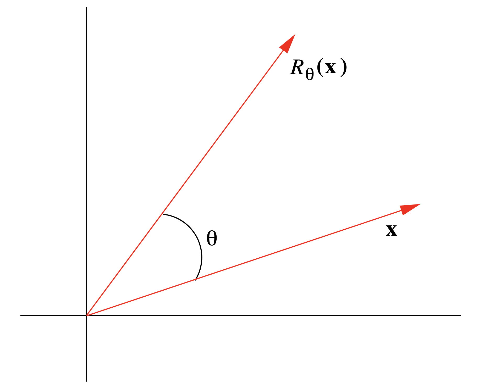
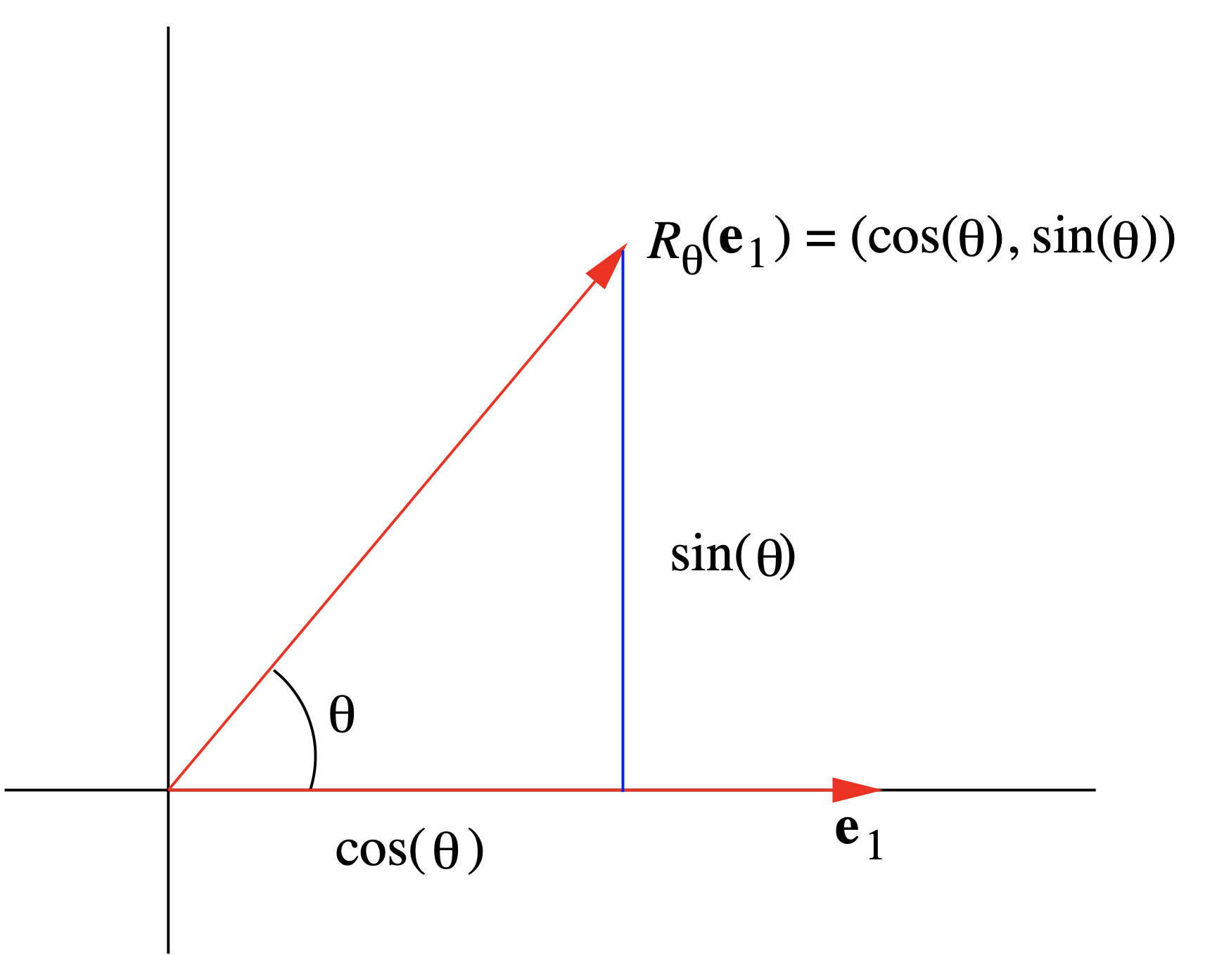
Dejar\(\begin{equation} R_{\theta}: \mathbb{R}^{2} \rightarrow \mathbb{R}^{2} \end{equation}\) ser la función que gira un vector\(\mathbf{x}\) en\(\mathbb{R}^2\) sentido antihorario a través de un ángulo θ, como se muestra en la Figura 1.5.1. Geométricamente, parece razonable que\(R_\theta\) sea una función lineal; es decir, rotar el vector\(\mathbf{x}+\mathbf{y} \) a través de un ángulo θ debería dar el mismo resultado que primero rotar\(\mathbf{x}\) y\(\mathbf{y}\) por separado a través de un ángulo θ y luego sumando, y girando un vector\(a \mathbf{x}\) a través de un ángulo θ debería dar el mismo resultado que primero rotar\( \mathbf{x}\) a través de un ángulo θ y luego multiplicar por\(a\). Ahora, a partir de la definición de\(\cos(\theta)\) y\(\sin(\theta)\),

\[ R_{\theta}\left(\mathbf{e}_{1}\right)=R_{\theta}(1,0)=(\cos (\theta), \sin (\theta)) \nonumber \]

(véase la Figura 1.5.2) y, dado que\(\mathbf{e}_{2}\) se\(\mathbf{e}_{1}\) gira, en sentido contrario a las agujas del reloj, en ángulo\(\frac{\pi}{2}\),

\[ R_{\theta}\left(\mathbf{e}_{2}\right)=R_{\theta+\frac{\pi}{2}}\left(\mathbf{e}_{1}\right)=\left(\cos \left(\theta+\frac{\pi}{2}\right), \sin \left(\theta+\frac{\pi}{2}\right)\right)=(-\sin (\theta), \cos (\theta)). \nonumber \]

De ahí

\ [R_ {\ theta} (x, y) =\ left [\ begin {array} {rr}
\ cos (\ theta) & -\ sin (\ theta)\\ sin (
\ theta)\\ sin (\ theta) &\ cos (
\ theta)\ end {array}\ derecha]\ left [\ begin {array} {l}
x\\
y
\ end {array}\ derecha]. \ label {1.5.12}\]

Figura\(\PageIndex{1}\): Rotación de un vector en el plano

Figura\(\PageIndex{2}\): Rotación\(\mathbf{e}_{1}\) a través de un ángulo θ

En el Ejercicio 9 se le pide verificar que la función lineal definida en (\(\ref{1.5.12}\)) de hecho gira vectores en un ángulo θ en sentido contrario a las agujas del reloj. Tenga en cuenta que, por ejemplo\(\theta=\frac{\pi}{2}\), cuando, tenemos

\ [R_ {\ frac {\ pi} {2}} (x, y) =\ left [\ begin {array} {rr}
0 & -1\\
1 & 0
\ end {array}\ right]\ left [\ begin {array} {l}
x\\
y
\ end {array}\ right]. \ nonumber\]

En particular, tenga en cuenta que\(R_{\frac{\pi}{2}}(1,0)=(0,1)\) y\(R_{\frac{\pi}{2}}(0,1)=(-1,0)\); es decir,\(R_{\frac{\pi}{2}}\) lleva\(\mathbf{e}_{1}\) a\(\mathbf{e}_{2}\) y\(\mathbf{e}_{2}\) a\(-\mathbf{e}_{1}\). Por otro ejemplo, si\(\theta=\frac{\pi}{6}\), entonces

\ [R_ {\ frac {\ pi} {6}} (x, y) =\ left [\ begin {array} {cc}
\ frac {\ sqrt {3}} {2} & -\ frac {1} {2}\
\ frac {1} {2} &\ frac {\ sqrt {3}} {2}
\ end {array}\ derecha] izquierda\ [\ begin {array} {l}
x\\
y
\ end {array}\ right]. \ nonumber\]

En particular,

\ [\ begin {ecuación}
R_ {\ frac {\ pi} {6}} (1,2) =\ left [\ begin {array} {cc}
\ frac {\ sqrt {3}} {2} & -\ frac {1} {2}\
\ frac {1}\\ frac {2} &\ frac {\ sqrt {3}} {2}
\ end {array} derecha]\ left [\ begin {array} {l}
1\\
2
\ end {array}\ derecha] =\ izquierda [\ begin {array} {c}
\ frac {\ sqrt {3}} {2} -1\\
\ frac {1} {2} +\ sqrt {3}
\ end {array}\ derecha] =\ izquierda [\ begin {array} {c}
\ frac {\ sqrt {3} -2} {2}\
\ frac {1+2\ sqrt {3}} {2}
\ end {array}\ right]
\ end {ecuación}. \ nonumber\]

Funciones afín

Definición\(\PageIndex{2}\)

Decimos que una función\(A: \mathbb{R}^{m} \rightarrow \mathbb{R}^{n}\) es afín si hay una función lineal\(L : \mathbb{R}^{m} \rightarrow \mathbb{R}^{n} \) y un vector\(\mathbf{b}\) en\(\mathbb{R}^n\) tal que

\[ A(\mathbf{x})=L(\mathbf{x})+\mathbf{b}\]

para todos\(\mathbf{x}\) en\( \mathbb{R}^m\).

Una función afín es solo una función lineal más una traducción. De nuestro conocimiento de las funciones lineales, se deduce que si\(A: \mathbb{R}^{m} \rightarrow \mathbb{R}^{n}\) es afín, entonces hay una\(n \times m\) matriz\(M\) y un vector\(\mathbf{b}\) en\(\mathbb{R}^n\) tal que

\[ A(\mathbf{x})=M \mathbf{x}+\mathbf{b}\]

para todos\(\mathbf{x}\) en\(\mathbb{R}^m\). En particular, si\(f: \mathbb{R} \rightarrow \mathbb{R}\) es afín, entonces hay números reales\(m\) y\(b\) tales que

\[ f(x)=m x+b\]

para todos los números reales\(x\).

Ejemplo\(\PageIndex{7}\)

La función

\[A(x, y)=(2 x+3, y-4 x+1) \nonumber \]

es una función afín desde\(\mathbb{R}^{2}\) hasta\(\mathbb{R}^{2}\) ya que podemos escribirla en la forma

\[ A(x, y)=L(x, y)+(3,1), \nonumber \]

donde\(L\) esta la función lineal

\[ L(x, y)=(2 x, y-4 x). \nonumber \]

Tenga en cuenta que\(L(1,0)=(2,-4)\) y\(L(0,1)=(0,1)\), por lo que también podemos escribir\(A\) en el formulario

\ [A (x, y) =\ left [\ begin {array} {rr}
2 & 0\\
-4 & 1
\ end {array}\ right]\ left [\ begin {array} {l}
x\\
y
\ end {array}\ right] +\ left [\ begin {array} {l}
3\\
1
\ end {array}\ right]. \ nonumber\]

Ejemplo\(\PageIndex{8}\)

La función afín

\ [A (x, y) =\ izquierda [\ begin {array} {cc}
\ frac {1} {\ sqrt {2}} & -\ frac {1} {\ sqrt {2}}\
\ frac {1} {\ sqrt {2}} &\ frac {1} {\ sqrt {2}}
\ end {array}\ derecha]\ izquierda [comenzar {array} {l}
x\\
y
\ end {array}\ right] +\ left [\ begin {array} {l}
1\\
2
\ end {array}\ derecha]\ nonumber\]

primero gira un vector, en sentido antihorario, en\(\mathbb{R}^{2}\) un ángulo de\(\frac{\pi}{4}\) y luego lo traduce por el vector\( (1,2) \).