2.3.E: Movimiento a lo largo de una curva (Ejercicios)

Ejercicio\(\PageIndex{1}\)

Para cada una de las siguientes, supongamos que una partícula se está moviendo a lo largo de una curva para que su posición en el tiempo\(t\) sea dada por\(\mathbf{x}=f(t)\). Encuentra la velocidad y aceleración de la partícula.

a)\(f(t)=\left(t^{2}+3, \sin (t)\right)\)

b)\(f(t)=\left(t^{2} e^{-2 t}, t^{3} e^{-2 t}, 3 t\right)\)

c)\(f(t)=\left(\cos \left(3 t^{2}\right), \sin \left(3 t^{2}\right)\right)\)

d)\(f(t)=\left(t \cos \left(t^{2}\right), t \sin \left(t^{2}\right), 3 t \cos \left(t^{2}\right)\right)\)

Responder

a)\(\mathbf{v}=(2 t, \cos (t)) ; \mathbf{a}=(2,-\sin (t)\)

c)\(\mathbf{v}=\left(-6 t \sin \left(3 t^{2}\right), 6 t \cos \left(3 t^{2}\right)\right)\);\(\mathbf{a}=\left(-36 t^{2} \cos \left(3 t^{2}\right)-6 \sin \left(3 t^{2}\right),-36 t^{2} \sin \left(3 t^{2}\right)+6 \cos \left(3 t^{2}\right)\right)\)

Ejercicio\(\PageIndex{2}\)

Encuentra la curvatura de las siguientes curvas en el punto dado.

a)\(f(t)=\left(t, t^{2}\right), t=1\)

b)\(f(t)=(3 \cos (t), \sin (t)), t=\frac{\pi}{4}\)

c)\(f(t)=(\cos (t), \sin (t), t), t=\frac{\pi}{3}\)

d)\(f(t)=\left(\cos (t), \sin (t), e^{-t}\right), t=0\)

Responder

a)\(\frac{2}{5 \sqrt{5}}\)

c)\(\frac{1}{2}\)

Ejercicio\(\PageIndex{3}\)

Trazar la curvatura para cada una de las siguientes curvas en el intervalo dado\(I\).

a)\(f(t)=\left(t, t^{2}\right), I=[-2,2]\)

b)\(f(t)=(\cos (t), 3 \sin (t)), I=[0,2 \pi]\)

c)\(g(t)=((1+2 \cos (t)) \cos (t),(1+2 \cos (t)) \sin (t)), I=[0,2 \pi]\)

d)\(h(t)=(2 \cos (t), \sin (t), 2 t), I=[0,2 \pi] \)

e)\(f(t)=(4 \cos (t)+\sin (4 t), 4 \sin (t)+\sin (4 t)), I=[0,2 \pi]\)

Ejercicio\(\PageIndex{4}\)

Para cada una de las siguientes, supongamos que una partícula se está moviendo a lo largo de una curva para que su posición en el tiempo\(t\) sea dada por\(\mathbf{x}=f(t)\). Encuentre las coordenadas de aceleración en la dirección del vector tangente unitario y en la dirección del vector normal de la unidad principal en el punto especificado. Escriba la aceleración como una suma de múltiplos escalares del vector tangente unitario y el vector normal de la unidad principal.

a)\(f(t)=(\sin (t), \cos (t)), t=\frac{\pi}{3}\)

b)\(f(t)=(\cos (t), 3 \sin (t)), t=\frac{\pi}{4}\)

c)\(f(t)=\left(t, t^{2}\right), t=1\)

d)\(f(t)=(\sin (t), \cos (t), t), t=\frac{\pi}{3}\)

Responder

a)\(a_{T}=0 ; a_{N}=1 ; a\left(\frac{\pi}{3}\right)=N\left(\frac{\pi}{3}\right)\)

c)\(a_{T}=\frac{4}{\sqrt{5}} ; a_{N}=\frac{2}{\sqrt{5}} ; a(1)=\frac{4}{\sqrt{5}} T(1)+\frac{2}{\sqrt{5}} N(1)\)

Ejercicio\(\PageIndex{5}\)

Supongamos que una partícula se mueve a lo largo\(C\) de una curva de\(\mathbb{R}^{3}\) manera que su posición en el tiempo\(t\) viene dada por\(\mathbf{x}=f(t)\). Dejar\(\mathbf{v}\),\(s\), y\(\mathbf{a}\) denotar la velocidad, velocidad, y aceleración de la partícula, respectivamente, y dejar\(\boldsymbol{\kappa}\) ser la curvatura de\(C\).

a) Utilizando los hechos\(\mathbf{v}=s T(t)\) y

\[ \mathbf{a}=\frac{d s}{d t} T(t)+s^{2} \kappa N(t) , \nonumber \]

demostrar que\[ \mathbf{v} \times \mathbf{a}=s^{3} \kappa(T(t) \times N(t)) . \nonumber \]

b) Utilizar el resultado de la parte (a) para demostrar que

\[ \kappa=\frac{\|\mathbf{v} \times \mathbf{a}\|}{\|\mathbf{v}\|^{3}}. \nonumber \]

Ejercicio\(\PageIndex{6}\)

Dejar\(H\) ser la hélice en\(\mathbb{R}^{3}\) parametrizada por\(f(t)=(\cos (t), \sin (t), t)\). Usa el resultado del Ejercicio 5 para calcular la curvatura\(\boldsymbol{\kappa}\) de\(H\) para cualquier momento\(t\).

Responder

\( \frac{1}{2}\)

Ejercicio\(\PageIndex{7}\)

Dejar\(C\) ser la hélice elíptica en\(\mathbb{R}^{3}\) parametrizada por\(f(t)=(4 \cos (t), 2 \sin (t), t)\). Utilice el resultado del Ejercicio 5 para calcular la curvatura\(\boldsymbol{\kappa}\) de\(C\) at\(t=\frac{\pi}{4}\)

Responder

\(\frac{\sqrt{74}}{11 \sqrt{11}}\)

Ejercicio\(\PageIndex{8}\)

Dejar\(C\) ser la curva en la\(\mathbb{R}^{2}\) que se encuentra la gráfica de la función\(\varphi: \mathbb{R} \rightarrow \mathbb{R}\). Usa el resultado del Ejercicio 5 para mostrar que la curvatura de\(C\) en el punto\((t, \varphi(t))\) es

\[\kappa=\frac{\left|\varphi^{\prime \prime}(t)\right|}{\left(1+\left(\varphi^{\prime}(t)\right)^{2}\right)^{\frac{3}{2}}} . \nonumber \]

Ejercicio\(\PageIndex{9}\)

\(P\)Déjese ser la gráfica de\(f(t)=t^{2}\). Usa el resultado del Ejercicio 8 para encontrar la curvatura de\(P\) at (1, 1) y (2, 4).

Responder

\(\frac{2}{5 \sqrt{5}}\)y\(\frac{2}{17 \sqrt{17}}\)

Ejercicio\(\PageIndex{10}\)

\(C\)Déjese ser la gráfica de\(f(t)=t^{3}\). Usa el resultado del Ejercicio 8 para encontrar la curvatura de\(C\) at (1, 1) y (2, 8).

Ejercicio\(\PageIndex{11}\)

\(C\)Déjese ser la gráfica de\(g(t)=\sin (t)\). Usa el resultado del Ejercicio 8 para encontrar la curvatura de\(C\) at\(\left(\frac{\pi}{2}, 1\right)\) y\(\left(\frac{\pi}{4}, \frac{1}{\sqrt{2}}\right)\).

Responder

1 y\(\frac{2}{3 \sqrt{3}}\)

Ejercicio\(\PageIndex{12}\)

Para cada una de las siguientes, supongamos que una partícula se está moviendo a lo largo de una curva para que su posición en el tiempo\(t\) sea dada por\(\mathbf{x}=f(t)\). Encuentra la distancia recorrida por la partícula en el intervalo de tiempo dado.

a)\(f(t)=(\sin (t), 3 \cos (t)), I=[0,2 \pi]\)

b)\(f(t)=(\cos (\pi t), \sin (\pi t), 2 t), I=[0,4]\)

c)\(f(t)=\left(t, t^{2}\right), I=[0,2]\)

d)\(f(t)=(t \cos (t), t \sin (t)), I=[0,2 \pi]\)

e)\(f(t)=\left(\cos (2 \pi t), \sin (2 \pi t), 3 t^{2}, t\right), I=[0,1]\)

f)\(f(t)=\left(e^{-t} \cos (\pi t), e^{-t} \sin (\pi t)\right), I=[-2,2]\)

g)\(f(t)=(4 \cos (t)+\sin (4 t), 4 \sin (t)+\sin (4 t)), I=[0,2 \pi]\)

Responder

a)\(13.3649\)

c)\(\sqrt{17}+\frac{1}{4} \sinh ^{-1}(4) \approx 4.64678\)

e)\(\frac{1}{2} \sqrt{37+4 \pi^{2}}+\frac{1}{12}\left(1+4 \pi^{2}\right) \sinh ^{-1}\left(\frac{6}{\sqrt{1+4 \pi^{2}}}\right) \approx 7.20788\)

g)\(32.2744\)

Ejercicio\(\PageIndex{13}\)

Verificar que la circunferencia de un círculo de radio\(r\) sea\(2\pi r\).

Ejercicio\(\PageIndex{14}\)

La curva parametrizada por

\[ f(t)=(\sin (2 t) \cos (t), \sin (2 t) \sin (t)) \nonumber \]

tiene cuatro “pétalos”. Encuentra la longitud de uno de estos pétalos.

Responder

2.4221

Ejercicio\(\PageIndex{15}\)

La curva\(C\) parametrizada por\(h(t)=\left(\cos ^{3}(t), \sin ^{3}(t)\right)\) se denomina hipocicloide (ver Figura 2.2.3 en la Sección 2.2). Encuentra la longitud de\(C\).

Contestar

6

Ejercicio\(\PageIndex{16}\)

Supongamos que\(\varphi: \mathbb{R} \rightarrow \mathbb{R}\) es continuamente diferenciable y deja\(C\) ser la parte de la gráfica de\(\varphi\) sobre el intervalo\([a,b]\). Demostrar que la longitud de\(C\) es

\[ \int_{a}^{b} \sqrt{1+\left(\varphi^{\prime}(t)\right)^{2}} d t . \nonumber \]

Ejercicio\(\PageIndex{17}\)

Usa el resultado del Ejercicio 16 para encontrar la longitud de un arco de la gráfica de\(f(t)= \sin (t)\).

Contestar

3.8202

Ejercicio\(\PageIndex{18}\)

Dejar\(h: \mathbb{R} \rightarrow \mathbb{R}^{n}\) parametrizar una curva\(C\). Decimos que\(C\) está parametrizado por la longitud del arco si es\(\|D h(t)\|=1\) para todos\(t\).

(a) Dejar\(\sigma\) ser la función de longitud de arco para\(C\) usar la parametrización\(f\) y dejar\(\sigma^{-1}\) ser su función inversa. Mostrar que la función\(g: \mathbb{R} \rightarrow \mathbb{R}^{n}\) definida por\(g(u)=f\left(\sigma^{-1}(u)\right)\) parametriza\(C\) por longitud de arco.

(b) Dejar\(C\) que la hélice circular entre\(\mathbb{R}^{3}\) con parametrización\(f(t)=(\cos (t), \sin (t), t)\). Encuentra una función\(g: \mathbb{R} \rightarrow \mathbb{R}^{n}\) que parametriza\(C\) por longitud de arco.

Ejercicio\(\PageIndex{19}\)

Supongamos que\(f: \mathbb{R} \rightarrow \mathbb{R}^{n}\) es continuo en el intervalo cerrado\([a,b]\) y tiene funciones de coordenadas\(f_{1}, f_{2}, \ldots, f_{n}\). Definimos la integral definida de f sobre el intervalo\([a,b]\) para ser

\[ \int_{a}^{b} f(t) d t=\left(\int_{a}^{b} f_{1}(t) d t, \int_{a}^{b} f_{2}(t) d t, \ldots, \int_{a}^{b} f_{n}(t) d t\right) . \nonumber \]

Mostrar que si una partícula se mueve así su velocidad en el tiempo\(t\) es\(\mathbf{v}(t)\), entonces, asumiendo que\(\mathbf{v}\) es una función continua en un intervalo\([a,b]\), la posición de la partícula para cualquier momento\(t\) en\([a,b]\) viene dada por

\[ \mathbf{x}(t)=\int_{a}^{t} \mathbf{v}(s) d s+\mathbf{x}(a) . \nonumber \]

Ejercicio\(\PageIndex{20}\)

Supongamos que una partícula se mueve a lo largo de una curva de\(\mathbb{R}^{3}\) manera que su velocidad en cualquier momento\(t\) es

\[ \mathbf{v}(t)=(\cos (2 t), \sin (2 t), 3 t) . \nonumber \]

Si la partícula está en (0, 1, 0) cuando\(t=0\), use el Ejercicio 19 para determinar su posición para cualquier otro momento\(t\).

Contestar

\(\mathbf{x}(t)=\left(\frac{1}{2} \sin (2 t), \frac{3}{2}-\frac{1}{2} \cos (2 t), \frac{3}{2} t^{2}\right)\)

Ejercicio\(\PageIndex{21}\)

Supongamos que una partícula se mueve a lo largo de una curva de\(\mathbb{R}^{3}\) manera que su aceleración en cualquier momento\(t\) es

\[ \mathbf{a}(t)=(\cos (t), \sin (t), 0) .\nonumber \]

Si la partícula está en (1, 2, 0) con la velocidad (0, 1, 1) a la vez\(t=0\), utilice el Ejercicio 19 para determinar su posición para cualquier otro momento\(t\).

Contestar

\(\mathbf{x}(t)=(2-\cos (t), 2+2 t-\sin (2 t), t)\)

Ejercicio\(\PageIndex{22}\)

Supongamos que un proyectil es disparado desde el suelo en un ángulo\(\alpha\) con una velocidad inicial\(v_0\), como se muestra en la Figura 2.3.5. Dejar\(\mathbf{x}(t)\),\(\mathbf{v}(t)\), y\(\mathbf{a}(t)\) ser la posición, velocidad y aceleración, respectivamente, del proyectil en el momento\(t\).

Figura\(\PageIndex{5}\): La trayectoria de un proyectil

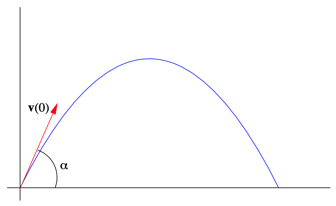
a) Explique por qué\(\mathbf{x}(0)=(0,0)\)\(\mathbf{v}(0)=\left(v_{0} \cos (\alpha), v_{0} \sin (\alpha)\right)\), y\(\mathbf{a}(t)=(0,-g)\) para todos\(t\), dónde\(g=9.8\) metros por segundo por segundo es la aceleración debida a la gravedad.

b) Utilice el Ejercicio 19 para encontrar\(\mathbf{v}(t)\).

(c) Utilice el Ejercicio 19 para encontrar\(\mathbf{x}(t)\).

(d) Demostrar que la curva parametrizada por\(\mathbf{x}(t)\) es una parábola. Es decir, dejar\(\mathbf{x}(t)=(x, y)\) y mostrar eso\(y=a x^{2}+b x+c\) para algunas constantes\(a\),\(b\), y\(c\).

e) Demostrar que el alcance del proyectil, es decir, la distancia horizontal recorrida, es

\[ R=\frac{v_{0} \sin (2 \alpha)}{g} \nonumber \]

y concluyen que el rango se maximiza cuando\(\alpha=\frac{\pi}{4}\)

f) ¿Cuándo choca el proyectil contra el suelo?

g) ¿Cuál es la altura máxima que alcanza el proyectil? ¿Cuándo alcanza esta altura?

Ejercicio\(\PageIndex{23}\)

Supongamos que\(\mathbf{a}_{1}, \mathbf{a}_{2}, \ldots, \mathbf{a}_{m}\) son vectores unitarios en\(\mathbb{R}^{n}\),\(m \leq n,\) que son mutuamente ortogonales (es decir,\(a_{i} \perp a_{j}\) cuándo\(i \neq j\)). Si\(\mathbf{x}\) es un vector en\(\mathbb{R}^{n}\) con

\[ \mathbf{x}=x_{1} \mathbf{a}_{1}+x_{2} \mathbf{a}_{2}+\cdots+x_{m} \mathbf{a}_{m} , \nonumber \]

demostrar eso\(x_{i}=\mathbf{x} \cdot \mathbf{a}_{i}, i=1,2, \ldots, m\).