4.4.E: Teorema de Green (Ejercicios)
- Page ID
- 111697
\( \newcommand{\vecs}[1]{\overset { \scriptstyle \rightharpoonup} {\mathbf{#1}} } \)
\( \newcommand{\vecd}[1]{\overset{-\!-\!\rightharpoonup}{\vphantom{a}\smash {#1}}} \)
\( \newcommand{\id}{\mathrm{id}}\) \( \newcommand{\Span}{\mathrm{span}}\)
( \newcommand{\kernel}{\mathrm{null}\,}\) \( \newcommand{\range}{\mathrm{range}\,}\)
\( \newcommand{\RealPart}{\mathrm{Re}}\) \( \newcommand{\ImaginaryPart}{\mathrm{Im}}\)
\( \newcommand{\Argument}{\mathrm{Arg}}\) \( \newcommand{\norm}[1]{\| #1 \|}\)
\( \newcommand{\inner}[2]{\langle #1, #2 \rangle}\)
\( \newcommand{\Span}{\mathrm{span}}\)
\( \newcommand{\id}{\mathrm{id}}\)
\( \newcommand{\Span}{\mathrm{span}}\)
\( \newcommand{\kernel}{\mathrm{null}\,}\)
\( \newcommand{\range}{\mathrm{range}\,}\)
\( \newcommand{\RealPart}{\mathrm{Re}}\)
\( \newcommand{\ImaginaryPart}{\mathrm{Im}}\)
\( \newcommand{\Argument}{\mathrm{Arg}}\)
\( \newcommand{\norm}[1]{\| #1 \|}\)
\( \newcommand{\inner}[2]{\langle #1, #2 \rangle}\)
\( \newcommand{\Span}{\mathrm{span}}\) \( \newcommand{\AA}{\unicode[.8,0]{x212B}}\)
\( \newcommand{\vectorA}[1]{\vec{#1}} % arrow\)
\( \newcommand{\vectorAt}[1]{\vec{\text{#1}}} % arrow\)
\( \newcommand{\vectorB}[1]{\overset { \scriptstyle \rightharpoonup} {\mathbf{#1}} } \)
\( \newcommand{\vectorC}[1]{\textbf{#1}} \)
\( \newcommand{\vectorD}[1]{\overrightarrow{#1}} \)
\( \newcommand{\vectorDt}[1]{\overrightarrow{\text{#1}}} \)
\( \newcommand{\vectE}[1]{\overset{-\!-\!\rightharpoonup}{\vphantom{a}\smash{\mathbf {#1}}}} \)
\( \newcommand{\vecs}[1]{\overset { \scriptstyle \rightharpoonup} {\mathbf{#1}} } \)
\( \newcommand{\vecd}[1]{\overset{-\!-\!\rightharpoonup}{\vphantom{a}\smash {#1}}} \)
\(\newcommand{\avec}{\mathbf a}\) \(\newcommand{\bvec}{\mathbf b}\) \(\newcommand{\cvec}{\mathbf c}\) \(\newcommand{\dvec}{\mathbf d}\) \(\newcommand{\dtil}{\widetilde{\mathbf d}}\) \(\newcommand{\evec}{\mathbf e}\) \(\newcommand{\fvec}{\mathbf f}\) \(\newcommand{\nvec}{\mathbf n}\) \(\newcommand{\pvec}{\mathbf p}\) \(\newcommand{\qvec}{\mathbf q}\) \(\newcommand{\svec}{\mathbf s}\) \(\newcommand{\tvec}{\mathbf t}\) \(\newcommand{\uvec}{\mathbf u}\) \(\newcommand{\vvec}{\mathbf v}\) \(\newcommand{\wvec}{\mathbf w}\) \(\newcommand{\xvec}{\mathbf x}\) \(\newcommand{\yvec}{\mathbf y}\) \(\newcommand{\zvec}{\mathbf z}\) \(\newcommand{\rvec}{\mathbf r}\) \(\newcommand{\mvec}{\mathbf m}\) \(\newcommand{\zerovec}{\mathbf 0}\) \(\newcommand{\onevec}{\mathbf 1}\) \(\newcommand{\real}{\mathbb R}\) \(\newcommand{\twovec}[2]{\left[\begin{array}{r}#1 \\ #2 \end{array}\right]}\) \(\newcommand{\ctwovec}[2]{\left[\begin{array}{c}#1 \\ #2 \end{array}\right]}\) \(\newcommand{\threevec}[3]{\left[\begin{array}{r}#1 \\ #2 \\ #3 \end{array}\right]}\) \(\newcommand{\cthreevec}[3]{\left[\begin{array}{c}#1 \\ #2 \\ #3 \end{array}\right]}\) \(\newcommand{\fourvec}[4]{\left[\begin{array}{r}#1 \\ #2 \\ #3 \\ #4 \end{array}\right]}\) \(\newcommand{\cfourvec}[4]{\left[\begin{array}{c}#1 \\ #2 \\ #3 \\ #4 \end{array}\right]}\) \(\newcommand{\fivevec}[5]{\left[\begin{array}{r}#1 \\ #2 \\ #3 \\ #4 \\ #5 \\ \end{array}\right]}\) \(\newcommand{\cfivevec}[5]{\left[\begin{array}{c}#1 \\ #2 \\ #3 \\ #4 \\ #5 \\ \end{array}\right]}\) \(\newcommand{\mattwo}[4]{\left[\begin{array}{rr}#1 \amp #2 \\ #3 \amp #4 \\ \end{array}\right]}\) \(\newcommand{\laspan}[1]{\text{Span}\{#1\}}\) \(\newcommand{\bcal}{\cal B}\) \(\newcommand{\ccal}{\cal C}\) \(\newcommand{\scal}{\cal S}\) \(\newcommand{\wcal}{\cal W}\) \(\newcommand{\ecal}{\cal E}\) \(\newcommand{\coords}[2]{\left\{#1\right\}_{#2}}\) \(\newcommand{\gray}[1]{\color{gray}{#1}}\) \(\newcommand{\lgray}[1]{\color{lightgray}{#1}}\) \(\newcommand{\rank}{\operatorname{rank}}\) \(\newcommand{\row}{\text{Row}}\) \(\newcommand{\col}{\text{Col}}\) \(\renewcommand{\row}{\text{Row}}\) \(\newcommand{\nul}{\text{Nul}}\) \(\newcommand{\var}{\text{Var}}\) \(\newcommand{\corr}{\text{corr}}\) \(\newcommand{\len}[1]{\left|#1\right|}\) \(\newcommand{\bbar}{\overline{\bvec}}\) \(\newcommand{\bhat}{\widehat{\bvec}}\) \(\newcommand{\bperp}{\bvec^\perp}\) \(\newcommand{\xhat}{\widehat{\xvec}}\) \(\newcommand{\vhat}{\widehat{\vvec}}\) \(\newcommand{\uhat}{\widehat{\uvec}}\) \(\newcommand{\what}{\widehat{\wvec}}\) \(\newcommand{\Sighat}{\widehat{\Sigma}}\) \(\newcommand{\lt}{<}\) \(\newcommand{\gt}{>}\) \(\newcommand{\amp}{&}\) \(\definecolor{fillinmathshade}{gray}{0.9}\)Ejercicio\(\PageIndex{1}\)
Dejado\(D\) ser el rectángulo cerrado adentro\(\mathbb{R}^2\) con vértices en (0, 0), (2, 0), (2, 4), y (0, 4), con límite\(\partial D\) orientado en sentido antihorario. Utilice el teorema de Green para evaluar las siguientes integrales de línea.
a)\(\int_{\partial D} 2 x y d x+3 x^{2} d y\)
b)\(\int_{\partial D} y d x+x d y\)
- Responder
-
a)\(\int_{\partial D} 2 x y d x+3 x^{2} d y=80\)
Ejercicio\(\PageIndex{2}\)
Dejado\(D\) ser el triángulo adentro\(\mathbb{R}^2\) con vértices en (0, 0), (2, 0), y (0, 4), con límite\(\partial D\) orientado en sentido antihorario. Utilice el teorema de Green para evaluar las siguientes integrales de línea.
a)\(\int_{\partial D} 2 x y^{2} d x+4 x d y\)
b)\(\int_{\partial D} y d x+x d y\)
c)\(\int_{\partial D} y d x-x d y\)
- Responder
-
a)\(\int_{\partial D} 2 x y^{2} d x+4 x d y=\frac{16}{3} \text { (c) } \int_{\partial D} y d x-x d y=-8\)
Ejercicio\(\PageIndex{3}\)
Usa el teorema de Green para encontrar el área de un círculo de radio\(r\).
Ejercicio\(\PageIndex{4}\)
Usa el teorema de Green para encontrar el área de la región\(D\) encerrada por el hipocicloide
\[ x^{\frac{2}{3}}+y^{\frac{2}{3}}=a^{\frac{2}{3}} , \nonumber \]
donde\(a > 0\). Tenga en cuenta que podemos parametrizar esta curva usando
\[ \varphi(t)=\left(a \cos ^{3}(t), a \sin ^{3}(t)\right) , \nonumber \]
\(0 \leq t \leq 2 \pi\).
- Responder
-
\(\frac{3}{8} \pi a^{2}\)
Ejercicio\(\PageIndex{5}\)
Usa el teorema de Green para encontrar el área de la región encerrada por un “pétalo” de la curva parametrizada por
\[ \varphi(t)=(\sin (2 t) \cos (t), \sin (2 t) \sin (t)) . \nonumber \]
- Responder
-
\(\frac{\pi}{8}\)
Ejercicio\(\PageIndex{6}\)
Encuentra el área de la región encerrada por el cardioide parametrizado por
\[ \varphi(t)=((2+\cos (t)) \cos (t),(2+\cos (t)) \sin (t)) , \nonumber \]
\(0 \leq t \leq 2 \pi\).
- Responder
-
\(\frac{9 \pi}{2}\)
Ejercicio\(\PageIndex{7}\)
Verificar (4.4.23), completando así la prueba del teorema de Green.
Ejercicio\(\PageIndex{8}\)
Supongamos que el campo vectorial\(F: \mathbb{R}^{2} \rightarrow \mathbb{R}^{2}\) con funciones de coordenadas\(p=F_{1}(x, y)\) y\(q=F_{2}(x, y)\) está\(C^1\) en un conjunto abierto que contiene la región Tipo III\(D\). Además, supongamos que\(F\) es el gradiente de una función escalar\(f: \mathbb{R}^{2} \rightarrow \mathbb{R}\).
a) Demostrar que
\[ \frac{\partial q}{\partial x}-\frac{\partial p}{\partial y}=0 \nonumber \]
para todos los puntos\((x,y)\) en\(D\).
b) Utilizar el teorema de Green para demostrar que
\[ \int_{\partial D} p d x+q d y=0 , \nonumber \]
donde\(\partial D\) es el límite de\(D\) con orientación en sentido antihorario.
Ejercicio\(\PageIndex{9}\)
¿Cuántas formas conoces para calcular el área de un círculo?
Ejercicio\(\PageIndex{10}\)
¿Quién era George Green?
Ejercicio\(\PageIndex{11}\)
Explicar cómo el teorema de Green es una generalización del Teorema Fundamental del Cálculo Integral.
Ejercicio\(\PageIndex{12}\)
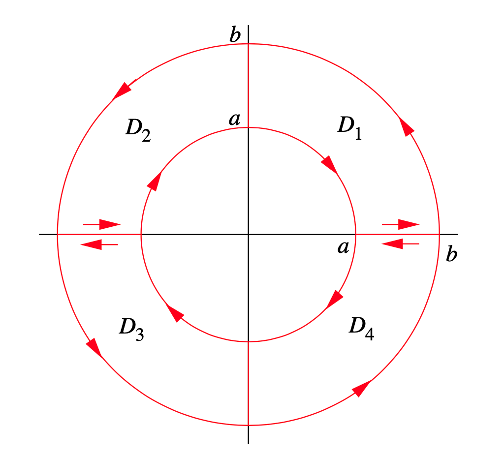
Dejar\(b > a\), dejar\(C_1\) ser el círculo de radio\(b\) centrado en el origen, y dejar\(C_2\) ser el círculo de radio\(a\) centrado en el origen. Si\(D\) es la región anular entre\(C_1\) y\(C_2\) y\(F\) es un campo\(C^1\) vectorial con funciones de coordenadas\(p=F_{1}(x, y)\) y\(q=F_{2}(x, y)\), mostrar que
\[ \iint_{D}\left(\frac{\partial q}{\partial x}-\frac{\partial p}{\partial y}\right) d x d y=\int_{C_{1}} p d x+q d y+\int_{C_{2}} p d x+q d y , \nonumber \]
donde\(C_1\) está orientado en sentido contrario a las agujas del reloj y\(C_2\) está orientado en el sentido de las agujas del reloj. (Pista: Descomponerse\(D\) en regiones Tipo III\(D_1\),\(D_2\), y\(D_3\)\(D_4\), cada una con límite orientado en sentido antihorario, como se muestra en la Figura 4.4.5.)
