1.2: Álgebra vectorial

Ahora que sabemos qué son los vectores, podemos comenzar a realizar algunas de las operaciones algebraicas habituales sobre ellos (por ejemplo, suma, resta). Antes de hacer eso, introduciremos la noción de escalar.

Definición 1.3

Un escalar es una cantidad que puede ser representada por un solo número.

Para nuestros propósitos, los escalares siempre serán números reales. El término escalar fue inventado por el matemático, físico y astrónomo irlandés del\(19^{th}\) siglo William Rowan Hamilton, para transmitir el sentido de algo que podría ser representado por un punto en una escala o gobernante graduado. La palabra vector proviene del latín, donde significa “portador”. Ejemplos de cantidades escalares son la masa, la carga eléctrica y la velocidad (no la velocidad). Ahora podemos definir la multiplicación escalar de un vector.

Definición 1.4

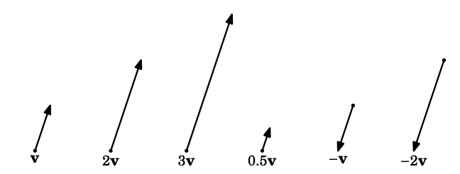
Para un vector escalar\(k\) y otro distinto de cero\(\textbf{v}\), el\(\textbf{scalar multiple}\) de\(\textbf{v}\) by\(k\), denotado por\(k\textbf{v}\), es el vector cuya magnitud es\(|k| \,\norm{\textbf{v}}\), apunta en la misma dirección que\(\textbf{v}\) si\(k > 0\), apunta en la dirección opuesta como\(\textbf{v}\) si\(k < 0\), y es el vector cero\(\textbf{0}\) si\(k = 0\). Para el vector cero\(\textbf{0}\), definimos\(k \textbf{0} = \textbf{0}\) para cualquier escalar\(k\).

Dos vectores\(\textbf{v}\) y\(\textbf{w}\) son\(\textbf{parallel}\) (denotados por\(\textbf{v} \parallel \textbf{w}\)) si uno es un múltiplo escalar del otro. Se puede pensar en la multiplicación escalar de un vector como estirar o reducir el vector, y como voltear el vector en la dirección opuesta si el escalar es un número negativo (Figura 1.2.1).

Figura 1.2.1

Recordemos que\(\textbf{translating}\) un vector distinto de cero significa que se cambia el punto inicial del vector pero se conservan la magnitud y dirección. Ahora estamos listos para definir el\(\textit{sum}\) de dos vectores.

Definición 1.5

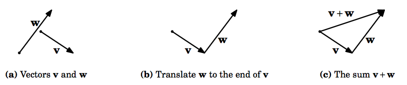
El\(\textbf{sum}\) de vectores\(\textbf{v}\) y\(\textbf{w}\), denotado por\(\textbf{v} + \textbf{w}\), se obtiene traduciendo de\(\textbf{w}\) manera que su punto inicial esté en el punto terminal de\(\textbf{v}\); el punto inicial de\(\textbf{v} + \textbf{w}\) es el punto inicial de\(\textbf{v}\), y su punto terminal es el nuevo punto terminal de \(\textbf{w}\).

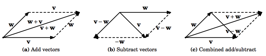
Intuitivamente, agregar\(\textbf{w}\) a\(\textbf{v}\) significa virar\(\textbf{w}\) al final de\(\textbf{v}\) (ver Figura 1.2.2).

Figura 1.2.2 Sumando vectores v y w

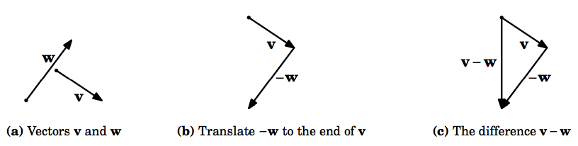
Observe que nuestra definición es válida para el vector cero (que es solo un punto, y por lo tanto se puede traducir), y así lo vemos\(\textbf{v} + \textbf{0} = \textbf{v} = \textbf{0} + \textbf{v}\) para cualquier vector\(\textbf{v}\). En particular,\(\textbf{0} + \textbf{0} = \textbf{0}\). Además, es fácil verlo\(\textbf{v} + (-\textbf{v}) = \textbf{0}\), como esperaríamos. En general, dado que el múltiplo escalar\(-\textbf{v} = -1 \,\textbf{v}\) es un vector bien definido, podemos definir de la\(\textbf{vector subtraction}\) siguiente manera:\(\textbf{v} - \textbf{w} = \textbf{v} + (-\textbf{w})\) (Figura 1.2.3).

Figura 1.2.3 Restar vectores v y w

La Figura 1.2.4 muestra el uso de “pruebas geométricas” de diversas leyes del álgebra vectorial, es decir, utiliza leyes de geometría elemental para probar afirmaciones sobre vectores. Por ejemplo, (a) muestra que\(\textbf{v} + \textbf{w} = \textbf{w} + \textbf{v}\) para cualquier vector\(\textbf{v}\),\(\textbf{w}\). Y (c) muestra cómo se puede pensar en\(\textbf{v} - \textbf{w}\) como el vector que está clavado al final de
\(\textbf{w}\) para sumar\(\textbf{v}\).

Figura 1.2.4 Álgebra vectorial “Geométrica”

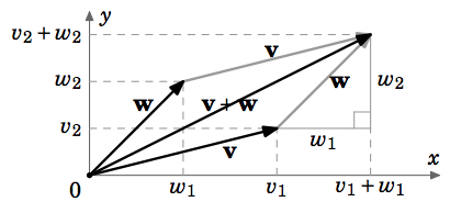
Observe que hemos abandonado temporalmente la práctica de iniciar vectores en el origen. De hecho, hasta el momento ni siquiera hemos mencionado coordenadas en esta sección. Dado que trataremos principalmente de coordenadas cartesianas en este libro, los siguientes dos teoremas son útiles para realizar álgebra vectorial en vectores en\(\mathbb{R}^{2}\) y\(\mathbb{R}^{3}\) comenzando en el origen.

Teorema 1.3

Dejar\(\textbf{v} = (v_{1}, v_{2})\),\(\textbf{w} = (w_{1}, w_{2})\) ser vectores adentro\(\mathbb{R}^{2}\), y dejar\(k\) ser un escalar. Entonces

1. \(k\textbf{v} = (kv_{1}, kv_{2})\)
2. \(\textbf{v + w} = (v_{1} + w_{1}, v_{2} + w_{2})\)

Prueba: a) Sin pérdida de generalidad, asumimos que\(v_{1}, v_{2} > 0\) (las otras posibilidades se manejan de manera similar). Si\(k = 0\) entonces\(k\textbf{v} = 0\textbf{v} = \textbf{0} = (0,0) = (0v_{1}, 0v_{2}) = (kv_{1}, kv_{2})\), que es lo que necesitábamos mostrar. Si\(k \ne 0\), entonces\((kv_{1}, kv_{2})\) yace sobre una línea con pendiente\(\frac{kv_{2}}{kv_{1}} = \frac{v_{2}}{v_{1}}\), que es la misma que la pendiente de la línea en la que se encuentra\(\textbf{v}\) (y por lo tanto\(k\textbf{v}\)), y\((kv_{1}, kv_{2})\) apunta en la misma dirección en esa línea que\(k\textbf{v}\). Además, por la fórmula (1.3) la magnitud de\((kv_{1}, kv_{2})\) es\(\sqrt{(kv_{1})^{2} + (kv_{2})^{2}} = \sqrt{k^{2} v_{1}^{2} + k^{2} v_{2}^{2}} = \sqrt{k^{2} (v_{1}^{2} + v_{2}^{2})} = |k| \,\sqrt{v_{1}^{2} + v_{2}^{2}} = |k| \,\norm{\textbf{v}}\). Entonces\(k\textbf{v}\) y\((kv_{1}, kv_{2})\) tienen la misma magnitud y dirección. Esto prueba (a).

(b) Sin pérdida de generalidad, suponemos que\(v_{1}, v_{2}, w_{1}, w_{2} > 0\) (las demás posibilidades se manejan de manera similar). De la Figura 1.2.5, vemos que al traducir\(\textbf{w}\) para iniciar al final de\(\textbf{v}\), el nuevo punto terminal de\(\textbf{w}\) es\((v_{1} + w_{1}, v_{2} + w_{2})\), por lo que por la definición de\(\textbf{v} + \textbf{w}\) este debe ser el punto terminal de\(\textbf{v} + \textbf{w}\). Esto prueba (b).

Figura 1.2.5

Teorema 1.4

Dejar\(\textbf{v} = (v_{1}, v_{2}, v_{3})\),\(\textbf{w} = (w_{1}, w_{2}, w_{3})\) ser vectores adentro\(\mathbb{R}^{3}\), dejar\(k\) ser un escalar. Entonces

1. \(k\textbf{v} = (kv_{1}, kv_{2}, kv_{3})\)
2. \(\textbf{v + w} = (v_{1} + w_{1}, v_{2} + w_{2}, v_{3} + w_{3})\)

El siguiente teorema resume las leyes básicas del álgebra vectorial.

Teorema 1.5

Para cualquier vector\(\textbf{u}, \textbf{v}, \textbf{w}\), y escalar\(k, l\),
tenemos

1. \(\textbf{v} + \textbf{w} = \textbf{w} + \textbf{v}\)Derecho Conmutativo
2. \(\textbf{u} + (\textbf{v} + \textbf{w}) = (\textbf{u} + \textbf{v}) + \textbf{w}\)Derecho asociativo
3. \(\textbf{v} + \textbf{0} = \textbf{v} = \textbf{0} + \textbf{v}\)Identidad Aditiva
4. \(\textbf{v} + (-\textbf{v}) = \textbf{0}\)Inverso Aditivo
5. \(k(l\textbf{v}) = (kl)\textbf{v}\)Derecho asociativo
6. \(k(\textbf{v} + \textbf{w}) = k\textbf{v} + k\textbf{w}\)Derecho Distributivo
7. \((k + l)\textbf{v} = k\textbf{v} + l\textbf{v}\)Derecho Distributivo

(a) Ya presentamos una prueba geométrica de esto en la Figura 1.2.4 (a).

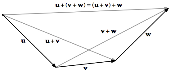
(b) Para ilustrar la diferencia entre pruebas analíticas y pruebas geométricas en álgebra vectorial, presentaremos aquí ambos tipos. Para la prueba analítica, utilizaremos vectores en\(\mathbb{R}^{3}\) (la prueba para\(\mathbb{R}^{2}\) es similar).

Dejemos\(\textbf{u} = (u_{1}, u_{2}, u_{3})\)\(\textbf{v} = (v_{1}, v_{2}, v_{3})\),,\(\textbf{w} = (w_{1}, w_{2}, w_{3})\) ser vectores en\(\mathbb{R}^{3}\). Entonces

\[\nonumber \begin{split}\textbf{u} + (\textbf{v} + \textbf{w}) &= (u_{1}, u_{2}, u_{3}) + ((v_{1}, v_{2}, v_{3}) + (w_{1}, w_{2}, w_{3})) \\[4pt] &= (u_{1}, u_{2}, u_{3}) + (v_{1} + w_{1}, v_{2} + w_{2}, v_{3} + w_{3}) \qquad \qquad &&\text{by Theorem 1.4 (b)} \\[4pt] &= (u_{1} + (v_{1} + w_{1}), u_{2} + (v_{2} + w_{2}), u_{3} + (v_{3} + w_{3})) &&\text{by Theorem 1.4 (b)} \\[4pt] &= ((u_{1} + v_{1}) + w_{1}, (u_{2} + v_{2}) + w_{2}, (u_{3} + v_{3}) + w_{3}) &&\text{by properties of real numbers} \\[4pt] &= (u_{1} + v_{1}, u_{2} + v_{2}, u_{3} + v_{3}) + (w_{1}, w_{2}, w_{3}) &&\text{by Theorem 1.4 (b)} \\[4pt] &= (\textbf{u} + \textbf{v}) + \textbf{w} \\[4pt] \end{split}\]

Esto completa la prueba analítica de (b). La Figura 1.2.6 proporciona la prueba geométrica.

Figura 1.2.6 Ley asociativa para la adición de vectores

c) Ya lo discutimos en la p.10.

d) Ya lo discutimos en la p.10.

(e) Demostraremos esto para un vector\(\textbf{v} = (v_{1}, v_{2}, v_{3})\) en\(\mathbb{R}^{3}\) (la prueba para\(\mathbb{R}^{2}\) es similar):

\[\nonumber \begin{split} k(l\textbf{v}) &= k(lv_{1}, lv_{2}, lv_{3}) \qquad & \text{by Theorem 1.4 (a)} \\[4pt] &= (klv_{1}, klv_{2}, klv_{3}) & \text{by Theorem 1.4 (a)} \\[4pt] &= (kl)(v_{1}, v_{2}, v_{3}) & \text{by Theorem 1.4 (a)} \\[4pt] &= (kl)\textbf{v} \\[4pt] \end{split}\]

f) y g): Dejado como ejercicios para el lector.

A\(\textbf{unit vector}\) es un vector con magnitud 1. Observe que para cualquier vector distinto de cero\(\textbf{v}\), el vector\(\frac{\textbf{v}}{\norm{\textbf{v}}}\) es un vector unitario que apunta en la misma dirección que\(\textbf{v}\), since\(\frac{1}{\norm{\textbf{v}}} > 0\) y
\(\norm{\frac{\textbf{v}}{\norm{\textbf{v}}}} = \frac{\norm{\textbf{v}}}{\norm{\textbf{v}}} = 1\). Dividir un vector distinto de cero\(\textbf{v}\) por a menudo\(\norm{\textbf{v}}\) se llama\(\textit{normalizing}\)\(\textbf{v}\).

Hay vectores unitarios específicos que usaremos a menudo, llamados\(\textbf{basis vectors}\):\(\textbf{i} = (1,0,0)\),\(\textbf{j} = (0,1,0)\), y\(\textbf{k} = (0,0,1)\) in\(\mathbb{R}^{3}\);\(\textbf{i} = (1,0)\) y\(\textbf{j} = (0,1)\) in\(\mathbb{R}^{2}\). Estos son útiles por varias razones: son mutuamente perpendiculares, ya que se encuentran en distintos ejes de coordenadas; todos son vectores unitarios:\(\norm{\textbf{i}} = \norm{\textbf{j}} = \norm{\textbf{k}} = 1\); cada vector puede escribirse como una combinación escalar única de los vectores base:\(\textbf{v} = (a,b) = a\,\textbf{i} + b\,\textbf{j}\) in\(\mathbb{R}^{2}\),\(\textbf{v} = (a,b,c) = a\,\textbf{i} + b\,\textbf{j} + c\,\textbf{k}\) in\(\mathbb{R}^{3}\). Ver Figura 1.2.7.

Figura 1.2.7 Vectores de base en diferentes dimensiones

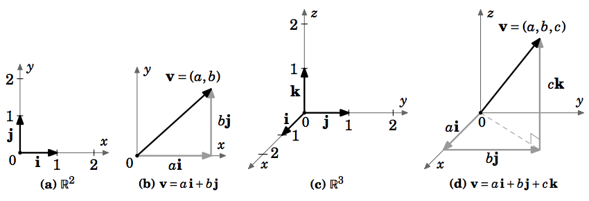
Cuando un vector\(\textbf{v} = (a,b,c)\) se escribe como\(\textbf{v} = a\,\textbf{i} + b\,\textbf{j} + c\,\textbf{k}\), decimos que\(\textbf{v}\) está en\(\textit{component form}\), y eso\(a\),\(b\), y\(c\) son los\(\textbf{i}\),\(\textbf{j}\), y\(\textbf{k}\) componentes, respectivamente, de\(\textbf{v}\). Contamos con:

\ begin {align*}
\ textbf {v} = v_ {1}\ textbf {i} + v_ {2}\ textbf {j} + v_ {3}\ textbf {k}, k\ text {a escalar} &\ Longrightarrow k\ textbf {v} = kv_ {1}\ textbf {i} + kv_ {2}\ textbf {j} + kv_ {3}\ textbf {k}\\ [4pt]
\ textbf {v} = v_ {1}\ textbf {i} + v_ {2}\ textbf {j} + v_ {3}\ textbf {k},\ textbf {w} = w_ {1}\ textbf {i} + w_ {2}\ textbf {j} + w_ {3}\ textbf {k} &\ Longrightarrow\ textbf {v} +\ textbf {w} =
(v_ {1} w_ {1})\ textbf {i} + (v_ {2} w_ {2})\ textbf {j} + (v_ {3} w_ {3})\ textbf {k}\\ [4pt]
\ textbf {v} = v_ {1}\ textbf {i} + v_ {2}\ textbf {j} + v_ {3}\ textbf {k} &\ Longrightarrow\ norm {\ textbf {v}} =
\ sqrt {v_ {1} ^ {2} + v_ {2} ^ {2} + v_ {3} ^ {2}}
\ end {align*}

Ejemplo 1.4

Dejar\(\textbf{v} = (2,1,-1)\) y\(\textbf{w} = (3,-4,2)\) entrar\(\mathbb{R}^{3}\).

1. Encontrar\(\textbf{v} - \textbf{w}\).
   \(\textit{Solution:}\)\(\textbf{v} - \textbf{w} = (2 - 3,1 - (-4), -1 - 2) = (-1,5,-3)\)
2. Encontrar\(3\textbf{v} + 2\textbf{w}\).
   \(\textit{Solution:}\)\(3\textbf{v} + 2\textbf{w} = (6,3,-3) + (6,-8,4) = (12,-5,1)\)
3. Escribir\(\textbf{v}\) y\(\textbf{w}\) en forma de componentes.
   \(\textit{Solution:}\)\(\textbf{v} = 2\,\textbf{i} + \textbf{j} - \textbf{k}\),\(\textbf{w} = 3\,\textbf{i} - 4\,\textbf{j} + 2\,\textbf{k}\)
4. Encuentra el vector\(\textbf{u}\) tal que\(\textbf{u} + \textbf{v} = \textbf{w}\).
   \(\textit{Solution:}\)Por Teorema 1.5\(\textbf{u} = \textbf{w} - \textbf{v} = -(\textbf{v} - \textbf{w}) = -(-1,5,-3) = (1,-5,3)\),, por parte (a).
5. Encuentra el vector\(\textbf{u}\) tal que\(\textbf{u} + \textbf{v} + \textbf{w} = \textbf{0}\).
   \(\textit{Solution:}\)Por teorema 1.5,\(\textbf{u} = -\textbf{w} - \textbf{v} = -(3,-4,2) - (2,1,-1) = (-5,3,-1)\).
6. Encuentra el vector\(\textbf{u}\) tal que\(2\textbf{u} + \textbf{i} - 2\,\textbf{j} = \textbf{k}\).
   \(\textit{Solution:}\)\(2\textbf{u} = -\textbf{i} + 2\,\textbf{j} + \textbf{k} \Longrightarrow \textbf{u} = -\frac{1}{2}\,\textbf{i} + \textbf{j} + \frac{1}{2}\,\textbf{k}\)
7. Encuentra el vector de unidad\(\frac{\textbf{v}}{\norm{\textbf{v}}}\).
   \(\textit{Solution:}\)\(\frac{\textbf{v}}{\norm{\textbf{v}}} = \frac{1}{\sqrt{2^{2} + 1^{2} + (-1)^{2}}} \,(2,1,-1) = \left(\frac{2}{\sqrt{6}},\frac{1}{\sqrt{6}},\frac{-1}{\sqrt{6}}\right)\)

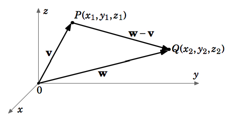
Ahora podemos probar fácilmente el Teorema 1.1 de la sección anterior. La distancia\(d\) entre dos puntos\(P = (x_{1}, y_{1}, z_{1})\) e\(Q = (x_{2}, y_{2}, z_{2})\) in\(\mathbb{R}^{3}\) es la misma que la longitud del vector\(\textbf{w} - \textbf{v}\), donde los vectores\(\textbf{v}\) y\(\textbf{w}\) se definen como\(\textbf{v} = (x_{1}, y_{1}, z_{1})\) y\(\textbf{w} = (x_{2}, y_{2}, z_{2})\) (ver Figura 1.2.8). Entonces desde\(\textbf{w} - \textbf{v} = (x_{2} - x_{1}, y_{2} - y_{1}, z_{2} - z_{1})\), entonces\(d = \norm{\textbf{w} - \textbf{v}} = \sqrt{(x_{2} - x_{1})^{2} + (y_{2} - y_{1})^{2} + (z_{2} - z_{1})^{2}}\) por el Teorema 1.2.

Figura 1.2.8 Prueba de Teorema 1.2:\(d = \norm{\textbf{w}−\textbf{v}}\)

Colaboradores y Atribuciones

• Template:ContribCorral