1.3: Producto Dot

Es posible que hayas notado que si bien definimos la multiplicación de un vector por un escalar en la sección anterior sobre álgebra vectorial, no definimos la multiplicación de un vector por un vector. Ahora veremos un tipo de multiplicación de vectores, llamado el producto punto.

Definición 1.6: Producto Dot

Let\(\textbf{v} = (v_{1}, v_{2}, v_{3})\) y\(\textbf{w}\) =\((w_{1}, w_{2}, w_{3})\) ser vectores en\(\mathbb{R}^{3}\). El\(\textbf{dot product}\) de\(\textbf{v}\) y\(\textbf{w}\), denotado por\(\textbf{v} \cdot \textbf{w}\), viene dado por:

\[\textbf{v} \cdot \textbf{w} = v_{1}w_{1} + v_{2}w_{2} + v_{3}w_{3}\]

Del mismo modo, para vectores\(\textbf{v} = (v_{1}, v_{2})\) y\(\textbf{w} = (w_{1}, w_{2})\) en\(\mathbb{R}^{2}\), el producto punto es:

\[\textbf{v} \cdot \textbf{w} = v_{1}w_{1} + v_{2}w_{2}\]

Observe que el producto punto de dos vectores es un escalar, no un vector. Entonces la ley asociativa que sostiene para la multiplicación de números y para la adición de vectores (ver Teorema 1.5 (b), (e)), sí se\(\textit{not}\) sostiene para el producto punto de vectores. ¿Por qué? Porque para los vectores\(\textbf{u}\)\(\textbf{v}\),\(\textbf{w}\),, el producto punto\(\textbf{u} \cdot \textbf{v}\) es un escalar, y así no\((\textbf{u} \cdot \textbf{v}) \cdot \textbf{w}\) está definido ya que el lado izquierdo de ese producto punto (la parte entre paréntesis) es un escalar y no un vector.

Para vectores\(\textbf{v} = v_{1}\textbf{i} + v_{2}\textbf{j} + v_{3}\textbf{k}\) y\(\textbf{w} = w_{1}\textbf{i} + w_{2}\textbf{j} + w_{3}\textbf{k}\) en forma de componentes, el producto punto está quieto\(\textbf{v} \cdot \textbf{w} = v_{1}w_{1} + v_{2}w_{2} + v_{3}w_{3}\).

También observe que definimos el producto punto de manera analítica, es decir, haciendo referencia a coordenadas vectoriales. Existe una forma geométrica de definir el producto punto, que ahora desarrollaremos como consecuencia de la definición analítica.

Definición 1.7

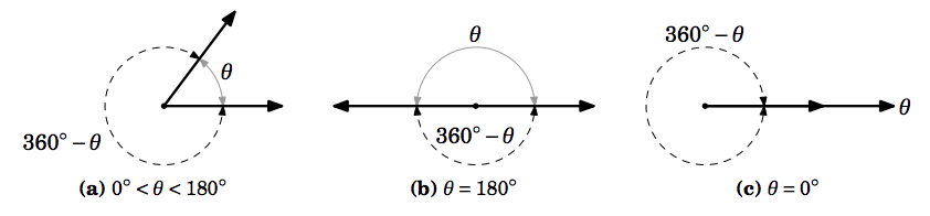
El\(\textbf{angle}\) entre dos vectores distintos de cero con el mismo punto inicial es el ángulo más pequeño entre ellos.

No definimos el ángulo entre el vector cero y cualquier otro vector. Cualquiera de dos vectores distintos de cero con el mismo punto inicial tienen dos ángulos entre ellos:\(\theta\) y\(360^{\circ} - \theta\). Siempre elegiremos el ángulo no negativo más pequeño\(\theta\) entre ellos, de modo que eso\(0^{\circ} \leq \theta \leq 180^{\circ}\). Ver Figura 1.3.1.

Figura 1.3.1 Ángulo entre vectores

Ahora podemos tomar una visión más geométrica del producto punto estableciendo una relación entre el producto punto de dos vectores y el ángulo entre ellos.

Teorema 1.6

Dejar\(\textbf{v}\),\(\textbf{w}\) ser vectores distintos de cero, y dejar que\(\theta\) sea el ángulo entre ellos. Entonces

\[\cos \theta = \dfrac{\textbf{v} \cdot \textbf{w}}{\norm{\textbf{v}}\, \norm{\textbf{w}}}\]

Prueba

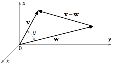
Demostraremos el teorema para vectores en\(\mathbb{R}^{3}\) (la prueba para\(\mathbb{R}^{2}\) es similar). Dejar\(\textbf{v} = (v_{1}, v_{2}, v_{3})\) y\(\textbf{w} = (w_{1}, w_{2}, w_{3})\). Por la Ley de Cosinos (ver Figura 1.3.2), tenemos

\[\norm{\textbf{v} - \textbf{w}}^{2} = \norm{\textbf{v}}^{2} + \norm{\textbf{w}}^{2} - 2\,\norm{\textbf{v}}\,\norm{\textbf{w}} \cos \theta \label{Equation 1.3.3}\]

(tenga en cuenta que Ecuación\(\ref{Equation 1.3.3}\)) sostiene incluso para los casos “degenerados”\(\theta = 0^{\circ}\) y\(180^{\circ}\)).

Figura 1.3.2

Ya que\(\textbf{v} - \textbf{w} = (v_{1} - w_{1}, v_{2} - w_{2}, v_{3} - w_{3})\), expandirse\(\norm{\textbf{v} - \textbf{w}}^{2}\) en Ecuación\(\ref{Equation 1.3.3}\) da

\[\nonumber \begin{align} \norm{\textbf{v}}^{2} + \norm{\textbf{w}}^{2} - 2\,\norm{\textbf{v}}\,\norm{\textbf{w}} \cos \theta &= (v_{1} - w_{1})^{2} + (v_{2} - w_{2})^{2} + (v_{3} - w_{3})^{2} \\[4pt] \nonumber&= (v_{1}^{2} - 2v_{1}w_{1} + w_{1}^{2}) + (v_{2}^{2} - 2v_{2}w_{2} +w_{2}^{2}) + (v_{3}^{2} - 2v_{3}w_{3} + w_{3}^{2}) \\[4pt] \nonumber&= (v_{1}^{2} + v_{2}^{2} + v_{3}^{2}) + (w_{1}^{2} + w_{2}^{2} + w_{3}^{2}) - 2(v_{1}w_{1} + v_{2}w_{2} + v_{3}w_{3}) \\[4pt] \nonumber&= \norm{\textbf{v}}^{2} + \norm{\textbf{w}}^{2} - 2(\textbf{v} \cdot \textbf{w}) \text{, so} \\[4pt] \nonumber -2\,\norm{\textbf{v}}\,\norm{\textbf{w}} \cos \theta &= -2(\textbf{v} \cdot \textbf{w}) \text{, so since }\textbf{v} \neq \textbf{0} \text{ and }\textbf{w} \neq \textbf{0} \text{ then} \\[4pt] \nonumber \cos \theta &= \dfrac{\textbf{v} \cdot \textbf{w}}{\norm{\textbf{v}} \norm{\textbf{w}}} \text{, since} \norm{\textbf{v}} > 0 \text{ and } \norm{\textbf{w}} > 0. \\[4pt] \end{align}\]

Ejemplo 1.5

Encuentra el ángulo\(\theta\) entre los vectores\(\textbf{v} = (2,1,-1)\) y\(\textbf{w} = (3,-4,1)\).

Solución

Desde\(\textbf{v} \cdot \textbf{w} = (2)(3) + (1)(-4) + (-1)(1) = 1\),\(\norm{\textbf{v}} = \sqrt{6}\), y\(\norm{\textbf{w}} = \sqrt{26}\), entonces

\[\cos \theta = \frac{\textbf{v} \cdot \textbf{w}}{\norm{\textbf{v}} \, \norm{\textbf{w}}} = \frac{1}{\sqrt{6}\,\sqrt{26}} = \frac{1}{2 \sqrt{39}} \approx 0.08 ~ \Longrightarrow ~ \theta = 85.41^{\circ}.\nonumber \]

Dos vectores distintos de cero son\(\textbf{perpendicular}\) si el ángulo entre ellos es\(90^{\circ}\). Ya que\(\cos 90^{\circ} = 0\), tenemos el siguiente corolario importante al Teorema 1.6:

Corolario 1.7

Dos vectores distintos de cero\(\textbf{v}\) y\(\textbf{w}\) son perpendiculares si y solo si\(\textbf{v} \cdot \textbf{w} = 0\).

Escribiremos\(\textbf{v} \perp \textbf{w}\) para indicarlo\(\textbf{v}\) y\(\textbf{w}\) son perpendiculares.

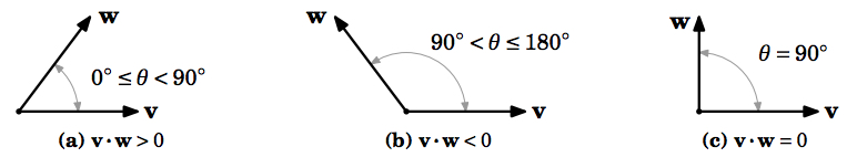
Desde\(\cos \theta > 0\) para\(0^{\circ} \le \theta < 90^{\circ}\) y\(\cos \theta < 0\) para\(90^{\circ} < \theta \le 180^{\circ}\), también tenemos:

Corolario 1.8

Si\(\theta\) es el ángulo entre vectores distintos de cero\(\textbf{v}\) y\(\textbf{w}\), entonces

\[\nonumber \textbf{v} \cdot \textbf{w} \text{ is }= \begin{cases} > 0, & \text{for }0^{\circ} \leq \theta < 90^{\circ} \\[4pt] 0, & \text{for }\theta = 90^{\circ} \\[4pt] < 0, & \text{for } 90^{\circ} < \theta \leq 180^{\circ}\end{cases}\]

Por Corolario 1.8, el producto de punto se puede considerar como una forma de decir si el ángulo entre dos vectores es agudo, obtuso o un ángulo recto, dependiendo de si el producto de punto es positivo, negativo o cero, respectivamente. Ver Figura 1.3.3.

Figura 1.3.3 Signo del producto punto y ángulo entre vectores

Ejemplo 1.6

¿Son los vectores\(\textbf{v} = (-1,5,-2)\) y\(\textbf{w} = (3,1,1)\) perpendiculares?

Solución

Sí,\(\textbf{v} \perp \textbf{w}\) ya que\(\textbf{v} \cdot \textbf{w} = (-1)(3) + (5)(1) + (-2)(1) = 0\).

El siguiente teorema resume las propiedades básicas del producto punto.

Teorema 1.9: Propiedades Básicas del Producto Dot

Para cualquier vector\(\textbf{u}, \textbf{v}, \textbf{w}\), y escalar\(k\), tenemos

1. \(\textbf{v} \cdot \textbf{w} = \textbf{w} \cdot \textbf{v}\)Derecho Conmutativo
2. \((k\textbf{v}) \cdot \textbf{w} = \textbf{v} \cdot (k\textbf{w}) = k(\textbf{v} \cdot \textbf{w})\)Derecho asociativo
3. \(\textbf{v} \cdot \textbf{0} = 0 = \textbf{0} \cdot \textbf{v}\)
4. \(\textbf{u} \cdot (\textbf{v} + \textbf{w}) = \textbf{u} \cdot \textbf{v} + \textbf{u} \cdot \textbf{w}\)Derecho Distributivo
5. \((\textbf{u} + \textbf{v}) \cdot \textbf{w} = \textbf{u} \cdot \textbf{w} + \textbf{v} \cdot \textbf{w}\)Derecho Distributivo
6. \(|\textbf{v} \cdot \textbf{w}| \le \norm{\textbf{v}}\,\norm{\textbf{w}}\)Desigualdad de Cauchy-Schwarz

Prueba

Las pruebas de las partes (a) - (e) son aplicaciones directas de la definición del producto punto, y se dejan al lector como ejercicios. Demostraremos la parte (f).

f) Si cualquiera\(\textbf{v} = \textbf{0}\) o\(\textbf{w} = \textbf{0}\), entonces\(\textbf{v} \cdot \textbf{w} = 0\) por la parte (c), y así la desigualdad se mantiene trivialmente. Entonces supongamos que\(\textbf{v}\) y\(\textbf{w}\) son vectores distintos de cero. Luego por el Teorema 1.6,

\[\nonumber \begin{align} \textbf{v} \cdot \textbf{w} &= \cos \theta\,\norm{\textbf{v}}\,\norm{\textbf{w}}\text{, so} \\[4pt] \nonumber |\textbf{v} \cdot \textbf{w}| &= |\cos \theta| \, \norm{\textbf{v}}\,\norm{\textbf{w}} \text{, so} \\[4pt] \nonumber |\textbf{v} \cdot \textbf{w}| &\le \norm{\textbf{v}}\,\norm{\textbf{w}} \text{ since }|\cos \theta| \le 1. \\[4pt] \end{align}\]

Usando el Teorema 1.9, vemos que si\(\textbf{u} \cdot \textbf{v} = 0\) y\(\textbf{u} \cdot \textbf{w} = 0\), entonces\(\textbf{u} \cdot (k\textbf{v} + l\textbf{w}) = k(\textbf{u} \cdot \textbf{v}) + l(\textbf{u} \cdot \textbf{w}) = k(0) + l(0) =0\) para todos los escalares\(k, l\). Así, tenemos el siguiente hecho:

\[\nonumber \text{If \(\textbf{u} \perp \textbf{v}\) and \(\textbf{u} \perp \textbf{w}\), then \(\textbf{u} \perp (k\textbf{v} + l\textbf{w})\) for all scalars \(k, l\).}\]

Para vectores\(\textbf{v}\) y\(\textbf{w}\), la colección de todas las combinaciones escalares\(k\textbf{v} + l\textbf{w}\) se llama\(\textbf{span}\) of\(\textbf{v}\) y\(\textbf{w}\). Si los vectores distintos de cero\(\textbf{v}\) y\(\textbf{w}\) son paralelos, entonces su span es una línea; si no son paralelos, entonces su span es un plano. Entonces lo que mostramos anteriormente es que un vector que es perpendicular a otros dos vectores también es perpendicular a su lapso.

El producto punto puede ser utilizado para derivar propiedades de las magnitudes de los vectores, la más importante de las cuales es la\(\textit{Triangle Inequality}\), como se da en el siguiente teorema:

Teorema 1.10: Limitaciones de magnitud vectorial

Para cualquier vector\(\textbf{v}, \textbf{w}\), tenemos

1. \(\norm{\textbf{v}}^{2} = \textbf{v} \cdot \textbf{v}\)
2. \(\norm{\textbf{v} + \textbf{w}} \le \norm{\textbf{v}} + \norm{\textbf{w}}\)Desigualdad del triángulo
3. \(\norm{\textbf{v} - \textbf{w}} \ge \norm{\textbf{v}} - \norm{\textbf{w}}\)

Prueba: a
) Dejado como ejercicio para el lector.

(b) Por parte (a) y Teorema 1.9, tenemos
\ begin {align*}
\ norm {\ textbf {v} +\ textbf {w}} ^ {2} &= (\ textbf {v} +\ textbf {w})\ cdot (\ textbf {v} +\ textbf {w})
=\ textbf {v}\ cdot\ textbf {v} +\ textbf {v}\ cdot\ textbf {w} +\ textbf {w}\ cdot\ textbf {v} +
\ textbf {w}\ cdot\ textbf {w}\\ [4pt]
&=\ norm {\ textbf {v}} ^ {2} + 2 (\ textbf {v}\ cdot\ textbf {w}) +\ norm {\ textbf {w}} ^ {2}\ text {, así como\(a \le |a|\)
para cualquier número real\(a\), tenemos}\\ [4pt]
&\ le\ norma {\ textbf {v}} ^ {2} + 2\, |\ textbf {v}\ cdot\ textbf {w} | +\ norm {\ textbf {w}} ^ {2}
\ text {, así que por Teorema 1.9 (f) tenemos}\\ [4pt]
&\ le\ norm {\ textbf {v}} ^ {2} + 2\,\ norm {\ textbf {v}}\,\ norm {\ textbf {w}} +\ norm {\ textbf {w}} {2} =
(\ norm {\ textbf {v}} +\ norm {\ textbf {w}}) ^ {2}\ texto {y así}\\ [4pt]
\ norm {\ textbf {v} +\ textbf {w}} &\ le\ norm {\ textbf {v}} +\ norm {\ textbf {w}}
\ text {después de tomar raíces cuadradas de ambos lados, lo que demuestra (b).}
\ end {align*}

(c) Desde\(\textbf{v} = \textbf{w} + (\textbf{v} - \textbf{w})\) entonces\(\norm{\textbf{v}} = \norm{\textbf{w} + (\textbf{v} - \textbf{w})} \le \norm{\textbf{w}} + \norm{\textbf{v} - \textbf{w}}\) por el Triángulo Desigualdad, así restando\(\norm{\textbf{w}}\) de ambos lados da\(\norm{\textbf{v}} - \norm{\textbf{w}} \le \norm{\textbf{v} - \textbf{w}}\).

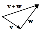
El Triángulo Desigualdad recibe su nombre por el hecho de que en cualquier triángulo, ningún lado es más largo que la suma de las longitudes de los otros dos lados (ver Figura 1.3.4). Otra forma de decir esto es con la familiar afirmación “la distancia más corta entre dos puntos es una línea recta”.

Figura 1.3.4

Colaboradores y Atribuciones

• Template:ContribCorral