1.4: Resumen y problemas adicionales
- Page ID
- 112526
\( \newcommand{\vecs}[1]{\overset { \scriptstyle \rightharpoonup} {\mathbf{#1}} } \)
\( \newcommand{\vecd}[1]{\overset{-\!-\!\rightharpoonup}{\vphantom{a}\smash {#1}}} \)
\( \newcommand{\id}{\mathrm{id}}\) \( \newcommand{\Span}{\mathrm{span}}\)
( \newcommand{\kernel}{\mathrm{null}\,}\) \( \newcommand{\range}{\mathrm{range}\,}\)
\( \newcommand{\RealPart}{\mathrm{Re}}\) \( \newcommand{\ImaginaryPart}{\mathrm{Im}}\)
\( \newcommand{\Argument}{\mathrm{Arg}}\) \( \newcommand{\norm}[1]{\| #1 \|}\)
\( \newcommand{\inner}[2]{\langle #1, #2 \rangle}\)
\( \newcommand{\Span}{\mathrm{span}}\)
\( \newcommand{\id}{\mathrm{id}}\)
\( \newcommand{\Span}{\mathrm{span}}\)
\( \newcommand{\kernel}{\mathrm{null}\,}\)
\( \newcommand{\range}{\mathrm{range}\,}\)
\( \newcommand{\RealPart}{\mathrm{Re}}\)
\( \newcommand{\ImaginaryPart}{\mathrm{Im}}\)
\( \newcommand{\Argument}{\mathrm{Arg}}\)
\( \newcommand{\norm}[1]{\| #1 \|}\)
\( \newcommand{\inner}[2]{\langle #1, #2 \rangle}\)
\( \newcommand{\Span}{\mathrm{span}}\) \( \newcommand{\AA}{\unicode[.8,0]{x212B}}\)
\( \newcommand{\vectorA}[1]{\vec{#1}} % arrow\)
\( \newcommand{\vectorAt}[1]{\vec{\text{#1}}} % arrow\)
\( \newcommand{\vectorB}[1]{\overset { \scriptstyle \rightharpoonup} {\mathbf{#1}} } \)
\( \newcommand{\vectorC}[1]{\textbf{#1}} \)
\( \newcommand{\vectorD}[1]{\overrightarrow{#1}} \)
\( \newcommand{\vectorDt}[1]{\overrightarrow{\text{#1}}} \)
\( \newcommand{\vectE}[1]{\overset{-\!-\!\rightharpoonup}{\vphantom{a}\smash{\mathbf {#1}}}} \)
\( \newcommand{\vecs}[1]{\overset { \scriptstyle \rightharpoonup} {\mathbf{#1}} } \)
\( \newcommand{\vecd}[1]{\overset{-\!-\!\rightharpoonup}{\vphantom{a}\smash {#1}}} \)
\(\newcommand{\avec}{\mathbf a}\) \(\newcommand{\bvec}{\mathbf b}\) \(\newcommand{\cvec}{\mathbf c}\) \(\newcommand{\dvec}{\mathbf d}\) \(\newcommand{\dtil}{\widetilde{\mathbf d}}\) \(\newcommand{\evec}{\mathbf e}\) \(\newcommand{\fvec}{\mathbf f}\) \(\newcommand{\nvec}{\mathbf n}\) \(\newcommand{\pvec}{\mathbf p}\) \(\newcommand{\qvec}{\mathbf q}\) \(\newcommand{\svec}{\mathbf s}\) \(\newcommand{\tvec}{\mathbf t}\) \(\newcommand{\uvec}{\mathbf u}\) \(\newcommand{\vvec}{\mathbf v}\) \(\newcommand{\wvec}{\mathbf w}\) \(\newcommand{\xvec}{\mathbf x}\) \(\newcommand{\yvec}{\mathbf y}\) \(\newcommand{\zvec}{\mathbf z}\) \(\newcommand{\rvec}{\mathbf r}\) \(\newcommand{\mvec}{\mathbf m}\) \(\newcommand{\zerovec}{\mathbf 0}\) \(\newcommand{\onevec}{\mathbf 1}\) \(\newcommand{\real}{\mathbb R}\) \(\newcommand{\twovec}[2]{\left[\begin{array}{r}#1 \\ #2 \end{array}\right]}\) \(\newcommand{\ctwovec}[2]{\left[\begin{array}{c}#1 \\ #2 \end{array}\right]}\) \(\newcommand{\threevec}[3]{\left[\begin{array}{r}#1 \\ #2 \\ #3 \end{array}\right]}\) \(\newcommand{\cthreevec}[3]{\left[\begin{array}{c}#1 \\ #2 \\ #3 \end{array}\right]}\) \(\newcommand{\fourvec}[4]{\left[\begin{array}{r}#1 \\ #2 \\ #3 \\ #4 \end{array}\right]}\) \(\newcommand{\cfourvec}[4]{\left[\begin{array}{c}#1 \\ #2 \\ #3 \\ #4 \end{array}\right]}\) \(\newcommand{\fivevec}[5]{\left[\begin{array}{r}#1 \\ #2 \\ #3 \\ #4 \\ #5 \\ \end{array}\right]}\) \(\newcommand{\cfivevec}[5]{\left[\begin{array}{c}#1 \\ #2 \\ #3 \\ #4 \\ #5 \\ \end{array}\right]}\) \(\newcommand{\mattwo}[4]{\left[\begin{array}{rr}#1 \amp #2 \\ #3 \amp #4 \\ \end{array}\right]}\) \(\newcommand{\laspan}[1]{\text{Span}\{#1\}}\) \(\newcommand{\bcal}{\cal B}\) \(\newcommand{\ccal}{\cal C}\) \(\newcommand{\scal}{\cal S}\) \(\newcommand{\wcal}{\cal W}\) \(\newcommand{\ecal}{\cal E}\) \(\newcommand{\coords}[2]{\left\{#1\right\}_{#2}}\) \(\newcommand{\gray}[1]{\color{gray}{#1}}\) \(\newcommand{\lgray}[1]{\color{lightgray}{#1}}\) \(\newcommand{\rank}{\operatorname{rank}}\) \(\newcommand{\row}{\text{Row}}\) \(\newcommand{\col}{\text{Col}}\) \(\renewcommand{\row}{\text{Row}}\) \(\newcommand{\nul}{\text{Nul}}\) \(\newcommand{\var}{\text{Var}}\) \(\newcommand{\corr}{\text{corr}}\) \(\newcommand{\len}[1]{\left|#1\right|}\) \(\newcommand{\bbar}{\overline{\bvec}}\) \(\newcommand{\bhat}{\widehat{\bvec}}\) \(\newcommand{\bperp}{\bvec^\perp}\) \(\newcommand{\xhat}{\widehat{\xvec}}\) \(\newcommand{\vhat}{\widehat{\vvec}}\) \(\newcommand{\uhat}{\widehat{\uvec}}\) \(\newcommand{\what}{\widehat{\wvec}}\) \(\newcommand{\Sighat}{\widehat{\Sigma}}\) \(\newcommand{\lt}{<}\) \(\newcommand{\gt}{>}\) \(\newcommand{\amp}{&}\) \(\definecolor{fillinmathshade}{gray}{0.9}\)No agregue manzanas a las naranjas: ¡Cada término en una ecuación o suma debe tener dimensiones idénticas! Esta restricción es una herramienta poderosa. Nos ayuda a evaluar integrales sin integrar y a predecir las soluciones de ecuaciones diferenciales. Aquí hay más problemas para practicar esta herramienta.
Problema 1.11 Integrales usando dimensiones
Utilice el análisis dimensional para encontrar\(\int_{0}^{\infty} e^{-ax}\) dx y\(\int\)\(\frac{dx}{x^{2}+a^{2}}\). Un resultado útil es
\[\int \frac{dx}{x^{2}+1} = arctanx + C. \label{1.20} \]
Problema 1.12 Ley Stefan—Boltzmann
La radiación de cuerpo negro es un fenómeno electromagnético, por lo que la intensidad de la radiación depende de la velocidad de la luz c. También es un fenómeno térmico, por lo que depende de la energía térmica\(k_{B}T\), donde\(T\) está la temperatura del objeto y\(k_{B}\) es la constante de Boltzmann. Y es un fenómeno cuántico, por lo que depende de la constante h de Planck. Así depende la intensidad de radiación de cuerpo negro I\(c\),\(k_{B}T\), y\(h\). Utilizar el análisis dimensional para mostrar eso\(I ∝ T^{4}\) y para encontrar la constante de proporcionalidad σ. Después busque la constante adimensional faltante. (Estos resultados se utilizan en la Sección 5.3.3.)
Problema 1.13 Arcoseno integral
Utilice el análisis dimensional para encontrar\(\int \sqrt{1 - 3x^{2}}\) dx. Un resultado útil es
\[\int \sqrt{1-x^{2}} dx =\frac{\arcsin x}{2}+\frac{x \sqrt{1-x^{2}}}{2}+C \label{1.21} \]
Problema 1.14 Tarifas relacionadas

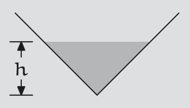
El agua se vierte en un cono invertido grande (con un ángulo de\(90^{◦}\) apertura) a una velocidad dV/dt =\(10m^{3}s^{-1}\). Cuando la profundidad del agua es\(h = 5\) m, estime la velocidad a la que aumenta la profundidad. Luego usa el cálculo para encontrar la tasa exacta.
Problema 1.15 Tercera ley de Kepler
La ley de la gravitación universal de Newton la famosa ley del cuadrado inverso dice que la fuerza gravitacional entre dos masas es
\[F = -\frac{Gm_{1}m_{2}}{r^{2}}, \label{1.22} \]
donde G es la constante de Newton,\(m_{1}\) y\(m_{2}\) son las dos masas, y r es su separación. Para un planeta orbitando el sol, la gravitación universal junto con la segunda ley de Newton da
\[m\frac{d^{2}r}{dt^{2}} = -\frac{GMm}{r^{2}} \hat{r}, \label{1.23} \]
Donde M es la masa del sol, m la masa del planeta, r es el vector del sol al planeta, y\(\hat{r}\) es el vector unitario en la dirección r.
¿Cómo depende el periodo orbital τ del radio orbital r? Busca la tercera ley de Kepler y compara tu resultado con ella.