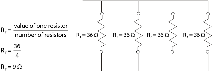
2.3: Circuitos paralelos

Última actualización
Guardar como PDF

Page ID: 152802

Camosun College
BCCampus (Download for free at http://open.bccampus.ca/find-open-textbooks)

\( \newcommand{\vecs}[1]{\overset { \scriptstyle \rightharpoonup} {\mathbf{#1}} } \) \( \newcommand{\vecd}[1]{\overset{-\!-\!\rightharpoonup}{\vphantom{a}\smash {#1}}} \)\(\newcommand{\id}{\mathrm{id}}\) \( \newcommand{\Span}{\mathrm{span}}\) \( \newcommand{\kernel}{\mathrm{null}\,}\) \( \newcommand{\range}{\mathrm{range}\,}\) \( \newcommand{\RealPart}{\mathrm{Re}}\) \( \newcommand{\ImaginaryPart}{\mathrm{Im}}\) \( \newcommand{\Argument}{\mathrm{Arg}}\) \( \newcommand{\norm}[1]{\| #1 \|}\) \( \newcommand{\inner}[2]{\langle #1, #2 \rangle}\) \( \newcommand{\Span}{\mathrm{span}}\) \(\newcommand{\id}{\mathrm{id}}\) \( \newcommand{\Span}{\mathrm{span}}\) \( \newcommand{\kernel}{\mathrm{null}\,}\) \( \newcommand{\range}{\mathrm{range}\,}\) \( \newcommand{\RealPart}{\mathrm{Re}}\) \( \newcommand{\ImaginaryPart}{\mathrm{Im}}\) \( \newcommand{\Argument}{\mathrm{Arg}}\) \( \newcommand{\norm}[1]{\| #1 \|}\) \( \newcommand{\inner}[2]{\langle #1, #2 \rangle}\) \( \newcommand{\Span}{\mathrm{span}}\)\(\newcommand{\AA}{\unicode[.8,0]{x212B}}\)

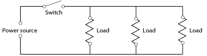
El circuito paralelo (Figura\(\PageIndex{1}\)) tiene características completamente diferentes. En un circuito paralelo, dos o más cargas están conectadas una al lado de la otra y son controladas por uno o más interruptores. Las diferentes cargas pueden tener cada una su propio interruptor, pero la diferencia principal es que cada una de las cargas tiene acceso a la misma cantidad de voltaje y puede operar independientemente de las demás. Hay más de un camino por el que puede fluir la corriente.

Figura\(\PageIndex{1}\): Circuito paralelo (CC BY-NC-SA; BC Industry Training Authority)

saf

Figura\(\PageIndex{2}\): Circuito paralelo (CC BY-NC-SA; BC Industry Training Authority)

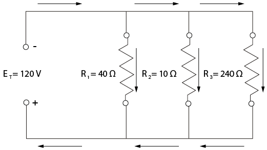
\[\begin{array}{l}{\mathrm{I}_{1}=\frac{\mathrm{E}_{1}}{\mathrm{R}_{1}}=\frac{120}{40}=3 \mathrm{amps}} \\ {\mathrm{I}_{2}=\frac{\mathrm{E}_{2}}{\mathrm{R}_{2}}=\frac{120}{10}=12 \mathrm{amps}} \\ {\mathrm{I}_{3}=\frac{\mathrm{E}_{3}}{\mathrm{R}_{3}}=\frac{120}{240}=0.5 \mathrm{amp}}\end{array}\]

\[R_{T}=\frac{E_{T}}{I_{T}}=\frac{120}{15.5}=7.7 \text { ohms }\]

\[R_{T}=\frac{1}{\frac{1}{R_{1}}+\frac{1}{R_{2}}+\frac{1}{R_{3}} \ldots}\]

\[\begin{aligned} R_{T}=& \frac{1}{\frac{1}{40}+\frac{1}{10}+\frac{1}{240}}=7.7 \text { ohms } \\ R_{T}=& \frac{1}{\frac{6}{240}+\frac{24}{240}+\frac{1}{240}} \\ R_{T}=& \frac{\frac{240}{240}}{31} \\ R_{T}=& 7.7 \text { ohms } \end{aligned}\]

Figura\(\PageIndex{3}\): Circuito paralelo con cuatro resistencias (CC BY-NC-SA; BC Industry Training Authority)

Figura\(\PageIndex{4}\): Circuito paralelo con dos resistencias (CC BY-NC-SA; BC Industry Training Authority)