2.7: Relaciones Kramers-Kroenig
- Page ID
- 84825

\( \newcommand{\vecs}[1]{\overset { \scriptstyle \rightharpoonup} {\mathbf{#1}} } \)
\( \newcommand{\vecd}[1]{\overset{-\!-\!\rightharpoonup}{\vphantom{a}\smash {#1}}} \)
\( \newcommand{\dsum}{\displaystyle\sum\limits} \)
\( \newcommand{\dint}{\displaystyle\int\limits} \)
\( \newcommand{\dlim}{\displaystyle\lim\limits} \)
\( \newcommand{\id}{\mathrm{id}}\) \( \newcommand{\Span}{\mathrm{span}}\)
( \newcommand{\kernel}{\mathrm{null}\,}\) \( \newcommand{\range}{\mathrm{range}\,}\)
\( \newcommand{\RealPart}{\mathrm{Re}}\) \( \newcommand{\ImaginaryPart}{\mathrm{Im}}\)
\( \newcommand{\Argument}{\mathrm{Arg}}\) \( \newcommand{\norm}[1]{\| #1 \|}\)
\( \newcommand{\inner}[2]{\langle #1, #2 \rangle}\)
\( \newcommand{\Span}{\mathrm{span}}\)
\( \newcommand{\id}{\mathrm{id}}\)
\( \newcommand{\Span}{\mathrm{span}}\)
\( \newcommand{\kernel}{\mathrm{null}\,}\)
\( \newcommand{\range}{\mathrm{range}\,}\)
\( \newcommand{\RealPart}{\mathrm{Re}}\)
\( \newcommand{\ImaginaryPart}{\mathrm{Im}}\)
\( \newcommand{\Argument}{\mathrm{Arg}}\)
\( \newcommand{\norm}[1]{\| #1 \|}\)
\( \newcommand{\inner}[2]{\langle #1, #2 \rangle}\)
\( \newcommand{\Span}{\mathrm{span}}\) \( \newcommand{\AA}{\unicode[.8,0]{x212B}}\)
\( \newcommand{\vectorA}[1]{\vec{#1}} % arrow\)
\( \newcommand{\vectorAt}[1]{\vec{\text{#1}}} % arrow\)
\( \newcommand{\vectorB}[1]{\overset { \scriptstyle \rightharpoonup} {\mathbf{#1}} } \)
\( \newcommand{\vectorC}[1]{\textbf{#1}} \)
\( \newcommand{\vectorD}[1]{\overrightarrow{#1}} \)
\( \newcommand{\vectorDt}[1]{\overrightarrow{\text{#1}}} \)
\( \newcommand{\vectE}[1]{\overset{-\!-\!\rightharpoonup}{\vphantom{a}\smash{\mathbf {#1}}}} \)
\( \newcommand{\vecs}[1]{\overset { \scriptstyle \rightharpoonup} {\mathbf{#1}} } \)
\(\newcommand{\longvect}{\overrightarrow}\)
\( \newcommand{\vecd}[1]{\overset{-\!-\!\rightharpoonup}{\vphantom{a}\smash {#1}}} \)
\(\newcommand{\ket}[1]{\left| #1 \right>}\)
\(\newcommand{\bra}[1]{\left< #1 \right|}\)
\(\newcommand{\braket}[2]{\left< #1 \vphantom{#2} \right| \left. #2 \vphantom{#1} \right>}\)
\(\newcommand{\braopket}[3]{\left< #1 \vphantom{#2}\vphantom{#3} \right| #2 \vphantom{#1}\vphantom{#3} \left| #3 \vphantom{#1}\vphantom{#2} \right>}\)
\(\newcommand{\qmvec}[1]{\mathbf{\vec{#1}}}\)
\(\newcommand{\op}[1]{\hat{\mathbf{#1}}}\)
\(\newcommand{\expect}[1]{\langle #1 \rangle}\)
\(\newcommand{\dfn}[1]{\emph{\textbf{#1}}}\)
La susceptibilidad lineal es la respuesta de frecuencia de un sistema lineal a un campo eléctrico aplicado, lo cual es causal, por lo que las partes reales e imaginarias obedecen a las Relaciones Kramers-Kroenig
\[\chi_r (\Omega) = \dfrac{2}{\pi} \int_{0}^{\infty} \dfrac{\omega \chi_i (\omega)}{\omega^2 - \Omega^2} d\omega = n^2 (\Omega) - 1, \nonumber \]
\[\chi_i (\Omega) = -\dfrac{2}{\pi} \int_{0}^{\infty} \dfrac{\Omega \chi_r (\omega)}{\omega^2 - \Omega^2} d\omega. \nonumber \]
En medios transparentes uno está operando lejos de las resonancias. Entonces la absorción o parte imaginaria de la susceptibilidad se puede aproximar por
\[\chi_i (\Omega) = \sum_i A_i \delta (\omega -\omega_i) \nonumber \]
y los resultados de la relación Kramers-Kroenig en una ecuación de Sellmeier para el índice de refracción
\[\begin{align*} n^2 (\Omega) &= 1 + \sum_i A_i \dfrac{\omega_i}{\omega_i^2 - \Omega^2} \\[4pt] &= 1 + \sum_i a_i \dfrac{\lambda}{\lambda^2 - \lambda_i^2} \end{align*} \nonumber \]
Para un ejemplo en el Cuadro 2.1 se muestran los coeficientes sellmeier para cuarzo fundido y zafiro.
| Cuarzo Fundido | Zafiro | |
|---|---|---|
| \(a_1\) | 0.6961663 | 1.023798 |
| \(a_2\) | 0.4079426 | 1.058364 |
| \(a_3\) | 0.8974794 | 5.280792 |
| \(\lambda_1^2\) | \(4.679148 \cdot 10^{-3}\) | \(3.77588 \cdot 10^{-3}\) |
| \(\lambda_2^2\) | \(1.3512063 \cdot 10^{-2}\) | \(1.22544 \cdot 10^{-2}\) |
| \(\lambda_3^2\) | \(0.9793400 \cdot 10^{2}\) | \(3.213616 \cdot 10^{2}\) |
Una situación típica para un material que tiene resonancias en los rayos UV e IR, tal como vidrio, se muestra en la Figura 2.12
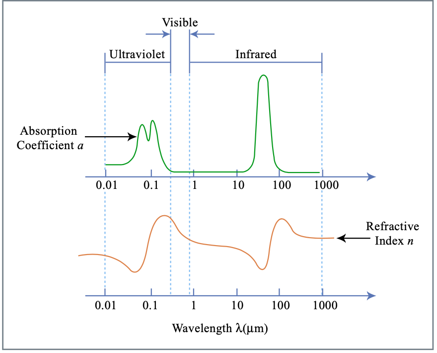
Las regiones donde el índice de refracción disminuye con la longitud de onda se suele llamar rango de dispersión normal y el comportamiento opuesto dispersión anormal
\[\begin{array} {rcl} {\dfrac{dn}{d\lambda}} & < & {\text{0: normal dispersion (blue refracts more than red)}} \\ {\dfrac{dn}{d\lambda}} & > & {\text{0: abnormal dispersion}} \end{array}\nonumber \]
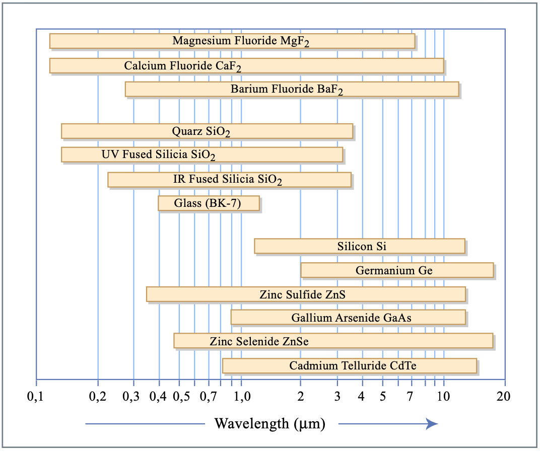
La Fig. 2.13 muestra el rango de transparencia de algunos medios de uso frecuente.