
8.3: Problemas en Vectores Aleatorios y Distribuciones Conjuntas


- Última actualización
- 31 oct 2022
- Guardar como PDF

( \newcommand{\kernel}{\mathrm{null}\,}\)
Ejercicio8.3.1
Se seleccionan dos cartas al azar, sin reemplazo, de una baraja estándar. XSea el número de ases yY sea el número de espadas. Bajo los supuestos habituales, determinar la distribución conjunta y los marginales.
- Contestar
-
XSea el número de ases yY sea el número de espadas. Definir los eventosASiAi,Si,, yNi,i=1,2 de dibujar as de espadas, otro as, pala (que no sea el as), y ninguno en la selección i. VamosP(i,k)=P(X=i,Y=k).
P(0,0)=P(N1N2)=3652⋅3551=12602652
P(0,1)=P(N1S2⋁S1N2)=3652⋅1251+1252⋅3651=8642652
P(0,2)=P(S1S2)=1252⋅1151=1322652
P(1, 0) = P(A_N_2 \bigvee N_1 S_2) = \dfrac{3}{52} \cdot \dfrac{36}{51} + \dfrac{36}{52} \cdot \dfrac{3}{51} = \dfrac{216}{2652}
P(1,1)=P(A1S2⋁S1A2⋁AS1N2⋁N1AS2)=352⋅1251+1252⋅351+152⋅3651+3652⋅151=1442652
P(1,2)=P(AS1S2⋁S1AS2)=152⋅1251+1252⋅151=242652
P(2,0)=P(A1A2)=352⋅251=62652
P(2,1)=P(AS1A2⋁A1AS2)=152⋅351+352⋅151=62652
P(2,2)=P(∅)=0
% type npr08_01
% file npr08_01.m
% Solution for Exercise 8.3.1.
X = 0:2;
Y = 0:2;
Pn = [132  24   0; 864 144  6; 1260 216 6];
P = Pn/(52*51);
disp('Data in Pn, P, X, Y')

npr08_01         % Call for mfile
Data in Pn, P, X, Y    % Result
PX = sum(P)
PX =  0.8507    0.1448    0.0045
PY = fliplr(sum(P'))
PY =  0.5588    0.3824    0.0588
Ejercicio8.3.2
Dos puestos para trabajos de campus están abiertos. Aplican dos estudiantes de segundo año, tres juniors y tres seniors. Se decide seleccionar dos al azar (cada par posible igualmente probable). XSea el número de alumnos de segundo año yY sea el número de juniors que sean seleccionados. Determinar la distribución conjunta para el par{X,Y} y a partir de esto determinar los marginales para cada uno.
- Contestar
-
DejenAi,Bi,Ci ser los eventos de seleccionar a un segundo, junior, o senior, respectivamente, en eli th juicio. DejarX ser el número de estudiantes de segundo año yY ser el número de juniors seleccionados.
SetP(i,k)=P(X=i,Y=k)
P(0,0)=P(C1C2)=38⋅27=656
P(0,1)=P(B1C2)+P(C1B2)=38⋅37+38⋅37=1856
P(0,2)=P(B1B2)=38⋅27=656
P(1,0)=P(A1C2)+P(C1A2)=28⋅37+38⋅27=1256
P(1,1)=P(A1B2)+P(B1A2)=28⋅37+38⋅27=1256
P(2,0)=P(A1A2)=28⋅17=256
P(1,2)=P(2,1)=P(2,2)=0
PX=[30/56 24/56 2/56]PY= [20/56 30/56 6/56]
% file npr08_02.m
% Solution for Exercise 8.3.2.
X = 0:2;
Y = 0:2;
Pn = [6 0 0; 18 12 0; 6 12 2];
P = Pn/56;
disp('Data are in X, Y,Pn, P')
npr08_02
Data are in X, Y,Pn, P
PX = sum(P)
PX =  0.5357    0.4286    0.0357
PY = fliplr(sum(P'))
PY =  0.3571    0.5357    0.1071
Ejercicio8.3.3
Se enrolla un dado. DejaX ser el número que aparece. Una moneda es volteadaX veces. YSea el número de cabezas que aparecen. Determinar la distribución conjunta para el par{X,Y}. AsumirP(X=k)=1/6 para1≤k≤6 y para cada unok,P(Y=j|X=k) tiene la distribución binomial (k, 1/2). Organizar la matriz conjunta como en el plano, con valores deY aumento hacia arriba. Determinar la distribución marginal paraY. (Para una forma basada en MATLAB de determinar la distribución conjunta, consulte el Ejemplo 14.1.7 de “Expectativa condicional, regresión”)
- Contestar
-
P(X=i,Y=k)=P(X=i)P(Y=k|X=i)=(1/6)P(Y=k|X=i).
% file npr08_03.m
% Solution for Exercise 8.3.3.
X = 1:6;
Y = 0:6;
P0 = zeros(6,7);       % Initialize
for i = 1:6            % Calculate rows of Y probabilities
    P0(i,1:i+1) = (1/6)*ibinom(i,1/2,0:i);
end
P = rot90(P0);         % Rotate to orient as on the plane
PY = fliplr(sum(P'));  % Reverse to put in normal order
disp('Answers are in X, Y, P, PY')
npr08_03            % Call for solution m-file
Answers are in X, Y, P, PY
disp(P)
         0         0         0         0         0    0.0026
         0         0         0         0    0.0052    0.0156
         0         0         0    0.0104    0.0260    0.0391
         0         0    0.0208    0.0417    0.0521    0.0521
         0    0.0417    0.0625    0.0625    0.0521    0.0391
    0.0833    0.0833    0.0625    0.0417    0.0260    0.0156
    0.0833    0.0417    0.0208    0.0104    0.0052    0.0026
disp(PY)
     0.1641  0.3125  0.2578  0.1667  0.0755  0.0208  0.0026
Ejercicio8.3.4
Como variación del Ejercicio 8.3.3. , Supongamos que se tira un par de dados en lugar de un solo dado. Determinar la distribución conjunta para el par{X,Y} y a partir de esto determinar la distribución marginal paraY.
- Contestar
-
% file npr08_04.m
% Solution for Exercise 8.3.4.
X = 2:12;
Y = 0:12;
PX = (1/36)*[1 2 3 4 5 6 5 4 3 2 1];
P0 = zeros(11,13);
for i = 1:11
    P0(i,1:i+2) = PX(i)*ibinom(i+1,1/2,0:i+1);
end
P = rot90(P0);
PY = fliplr(sum(P'));
disp('Answers are in X, Y, PY, P')
npr08_04
Answers are in X, Y, PY, P
disp(P)
  Columns 1 through 7
         0         0         0         0         0         0         0
         0         0         0         0         0         0         0
         0         0         0         0         0         0         0
         0         0         0         0         0         0         0
         0         0         0         0         0         0    0.0005
         0         0         0         0         0    0.0013    0.0043
         0         0         0         0    0.0022    0.0091    0.0152
         0         0         0    0.0035    0.0130    0.0273    0.0304
         0         0    0.0052    0.0174    0.0326    0.0456    0.0380
         0    0.0069    0.0208    0.0347    0.0434    0.0456    0.0304
    0.0069    0.0208    0.0312    0.0347    0.0326    0.0273    0.0152
    0.0139    0.0208    0.0208    0.0174    0.0130    0.0091    0.0043
    0.0069    0.0069    0.0052    0.0035    0.0022    0.0013    0.0005
  Columns 8 through 11
         0         0         0    0.0000
         0         0    0.0000    0.0001
         0    0.0001    0.0003    0.0004
    0.0002    0.0008    0.0015    0.0015
    0.0020    0.0037    0.0045    0.0034
    0.0078    0.0098    0.0090    0.0054
    0.0182    0.0171    0.0125    0.0063
    0.0273    0.0205    0.0125    0.0054
    0.0273    0.0171    0.0090    0.0034
    0.0182    0.0098    0.0045    0.0015
    0.0078    0.0037    0.0015    0.0004
    0.0020    0.0008    0.0003    0.0001
    0.0002    0.0001    0.0000    0.0000
disp(PY)
  Columns 1 through 7
    0.0269    0.1025    0.1823    0.2158    0.1954    0.1400    0.0806
  Columns 8 through 13
    0.0375    0.0140    0.0040    0.0008    0.0001    0.0000
Ejercicio8.3.5
Supongamos que se tira un par de dados. DejarX ser el número total de manchas que aparecen. Enrolle el par unaX vez más. YSea el número de sietes que se lanzan en losX rollos. Determinar la distribución conjunta para el par{X,Y} y a partir de esto determinar la distribución marginal paraY. ¿Cuál es la probabilidad de tres o más sietes?
- Contestar
-
% file npr08_05.m
% Data and basic calculations for Exercise 8.3.5.
PX = (1/36)*[1 2 3 4 5 6 5 4 3 2 1];
X = 2:12;
Y = 0:12;
P0 = zeros(11,13);
for i = 1:11
  P0(i,1:i+2) = PX(i)*ibinom(i+1,1/6,0:i+1);
end
P = rot90(P0);
PY = fliplr(sum(P'));
disp('Answers are in X, Y, P, PY')
npr08_05
Answers are in X, Y, P, PY
disp(PY)
  Columns 1 through 7
    0.3072    0.3660    0.2152    0.0828    0.0230    0.0048    0.0008
  Columns 8 through 13
    0.0001    0.0000    0.0000    0.0000    0.0000    0.0000
Ejercicio8.3.6
El par{X,Y} tiene la distribución conjunta (en m-file npr08_06.m):
X=[-2.3 -0.7 1.1 3.9 5.1]Y= = [1.3 2.5 4.1 5.3]
Determinar la distribución marginal y los valores de esquina paraFXY. DeterminarP(X+Y>2) yP(X≥Y).
- Contestar
-
npr08_06
Data are in X, Y, P
jcalc
Enter JOINT PROBABILITIES (as on the plane)  P
Enter row matrix of VALUES of X  X
Enter row matrix of VALUES of Y  Y
 Use array operations on matrices X, Y, PX, PY, t, u, and P
disp([X;PX]')
   -2.3000    0.2300
   -0.7000    0.1700
    1.1000    0.2000
    3.9000    0.2020
    5.1000    0.1980

disp([Y;PY]')
    1.3000    0.2980
    2.5000    0.3020
    4.1000    0.1900
    5.3000    0.2100
jddbn
Enter joint probability matrix (as on the plane)  P
To view joint distribution function, call for FXY
disp(FXY)
    0.2300    0.4000    0.6000    0.8020    1.0000
    0.1817    0.3160    0.4740    0.6361    0.7900
    0.1380    0.2400    0.3600    0.4860    0.6000
    0.0667    0.1160    0.1740    0.2391    0.2980
P1 = total((t+u>2).*P)
P1 =  0.7163
P2 = total((t>=u).*P)
P2 =  0.2799
Ejercicio8.3.7
El par{X,Y} tiene la distribución conjunta (en m-file npr08_07.m):
P(X=i,Y=u)
| t = | -3.1 | -0.5 | 1.2 | 2.4 | 3.7 | 4.9 |
| u = 7.5 | 0.0090 | 0.0396 | 0.0594 | 0.0216 | 0.0440 | 0.0203 |
| 4.1 | 0.0495 | 0 | 0.1089 | 0.0528 | 0.0363 | 0.0231 |
| -2.0 | 0.0405 | 0.1320 | 0.0891 | 0.0324 | 0.0297 | 0.0189 |
| -3.8 | 0.0510 | 0.0484 | 0.0726 | 0.0132 | 0 | 0.0077 |
Determinar las distribuciones marginales y los valores de esquina paraFXY. DeterminarP(1≤X≤4,Y>4) yP(|X−Y|≤2).
- Contestar
-
npr08_07
Data are in X, Y, P
jcalc
Enter JOINT PROBABILITIES (as on the plane)  P
Enter row matrix of VALUES of X  X
Enter row matrix of VALUES of Y  Y
 Use array operations on matrices X, Y, PX, PY, t, u, and P
disp([X;PX]')
   -3.1000    0.1500
   -0.5000    0.2200
    1.2000    0.3300
    2.4000    0.1200
    3.7000    0.1100
    4.9000    0.0700
disp([Y;PY]')
   -3.8000    0.1929
   -2.0000    0.3426
    4.1000    0.2706
    7.5000    0.1939
jddbn
Enter joint probability matrix (as on the plane)  P
To view joint distribution function, call for FXY
disp(FXY)
    0.1500    0.3700    0.7000    0.8200    0.9300    1.0000
    0.1410    0.3214    0.5920    0.6904    0.7564    0.8061
    0.0915    0.2719    0.4336    0.4792    0.5089    0.5355
    0.0510    0.0994    0.1720    0.1852    0.1852    0.1929
M = (1<=t)&(t<=4)&(u>4);
P1 = total(M.*P)
P1 =  0.3230
P2 = total((abs(t-u)<=2).*P)
P2 =  0.3357
Ejercicio8.3.8
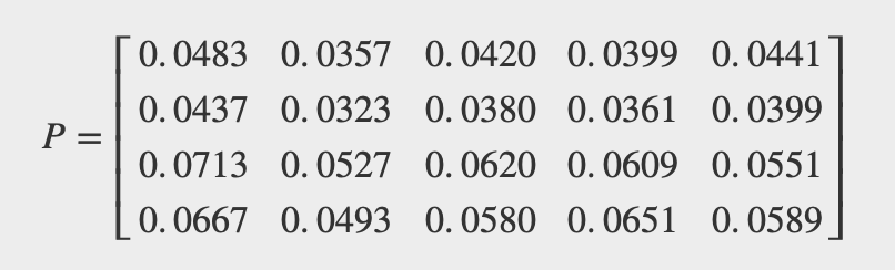
El par{X,Y} tiene la distribución conjunta (en m-file npr08_08.m):
P(X=t,Y=u)
| t = | 1 | 3 | 5 | 7 | 9 | 11 | 13 | 15 | 17 | 19 |
| u = 12 | 0.0156 | 0.0191 | 0.0081 | 0.0035 | 0.0091 | 0.0070 | 0.0098 | 0.0056 | 0.0091 | 0.0049 |
| 10 | 0.0064 | 0.0204 | 0.0108 | 0.0040 | 0.0054 | 0.0080 | 0.0112 | 0.0064 | 0.0104 | 0.0056 |
| 9 | 0.0196 | 0.0256 | 0.0126 | 0.0060 | 0.0156 | 0.0120 | 0.0168 | 0.0096 | 0.0056 | 0.0084 |
| 5 | 0.0112 | 0.0182 | 0.0108 | 0.0070 | 0.0182 | 0.0140 | 0.0196 | 0.0012 | 0.0182 | 0.0038 |
| 3 | 0.0060 | 0.0260 | 0.0162 | 0.0050 | 0.0160 | 0.0200 | 0.0280 | 0.0060 | 0.0160 | 0.0040 |
| -1 | 0.0096 | 0.0056 | 0.0072 | 0.0060 | 0.0256 | 0.0120 | 0.0268 | 0.0096 | 0.0256 | 0.0084 |
| -3 | 0.0044 | 0.0134 | 0.0180 | 0.0140 | 0.0234 | 0.0180 | 0.0252 | 0.0244 | 0.0234 | 0.0126 |
| -5 | 0.0072 | 0.0017 | 0.0063 | 0.0045 | 0.0167 | 0.0090 | 0.0026 | 0.0172 | 0.0217 | 0.0223 |
Determinar las distribuciones marginales. DeterminarFXY(10,6) yP(X>Y).
- Contestar
-
npr08_08
Data are in X, Y, P
jcalc
- - - - - - - - -
 Use array operations on matrices X, Y, PX, PY, t, u, and P
disp([X;PX]')
    1.0000    0.0800
    3.0000    0.1300
    5.0000    0.0900
    7.0000    0.0500
    9.0000    0.1300
   11.0000    0.1000
   13.0000    0.1400
   15.0000    0.0800
   17.0000    0.1300
   19.0000    0.0700
disp([Y;PY]')
   -5.0000    0.1092
   -3.0000    0.1768
   -1.0000    0.1364
    3.0000    0.1432
    5.0000    0.1222
    9.0000    0.1318
   10.0000    0.0886
   12.0000    0.0918
F = total(((t<=10)&(u<=6)).*P)
F =   0.2982
P = total((t>u).*P)
P =   0.7390
Ejercicio8.3.9
Se conservaron datos sobre el efecto del tiempo de capacitación en el tiempo para realizar un trabajo en una línea de producción. Xes la cantidad de entrenamiento, en horas, yY es el tiempo para realizar la tarea, en minutos. Los datos son los siguientes (en m-file npr08_09.m):
P(X=t,Y=u)
| t = | 1 | 1.5 | 2 | 2.5 | 3 |
| u = 5 | 0.039 | 0.011 | 0.005 | 0.001 | 0.001 |
| 4 | 0.065 | 0.070 | 0.050 | 0.015 | 0.010 |
| 3 | 0.031 | 0.061 | 0.137 | 0.051 | 0.033 |
| 2 | 0.012 | 0.049 | 0.163 | 0.058 | 0.039 |
| 1 | 0.003 | 0.009 | 0.045 | 0.025 | 0.017 |
Determinar las distribuciones marginales. DeterminarFXY(2,3) yP(Y/X≥1.25).
- Contestar
-
npr08_09
Data are in X, Y, P
jcalc
- - - - - - - - - - - -
 Use array operations on matrices X, Y, PX, PY, t, u, and P
disp([X;PX]')
    1.0000    0.1500
    1.5000    0.2000
    2.0000    0.4000
    2.5000    0.1500
    3.0000    0.1000
disp([Y;PY]')
    1.0000    0.0990
    2.0000    0.3210
    3.0000    0.3130
    4.0000    0.2100
    5.0000    0.0570
F = total(((t<=2)&(u<=3)).*P)
F =   0.5100
P = total((u./t>=1.25).*P)
P =   0.5570
Para las densidades articulares en los Ejercicios 10-22 a continuación
- Esbozar la región de definición y determinar analíticamente las funciones de densidad marginalfX yfY.
- Utilice una aproximación discreta para trazar la densidad marginalfX y la función de distribución marginalFX.
- Calcular analíticamente las probabilidades indicadas.
- Determinar por aproximación discreta las probabilidades indicadas.
Ejercicio8.3.10
fXY(t,u)=1para0≤t≤1,0≤u≤2(1−t).
P(X>1/2,Y>1),P(0≤X≤1/2,Y>1/2),P(Y≤X)
- Contestar
-
Región es triángulo con vértices (0, 0), (1, 0), (0, 2).
fX(t)=∫2(1−t)0du=2(1−t),0≤t≤1
fY(u)=∫1−u/20dt=1−u/2,0≤u≤2
M1={(t,u):t>1/2,u>1}yace fuera del trianlgeP((X,Y)∈M1)=0
M2={(t,u):0≤t≤1/2,u>1/2}tiene área en el triángulo = 1/2
M3= la región en el triángulo bajou=t, que tiene área 1/3
tuappr
Enter matrix [a b] of X-range endpoints  [0 1]
Enter matrix [c d] of Y-range endpoints  [0 2]
Enter number of X approximation points  200
Enter number of Y approximation points  400
Enter expression for joint density  (t<=1)&(u<=2*(1-t))
Use array operations on X, Y, PX, PY, t, u, and P
fx = PX/dx;
FX = cumsum(PX);
plot(X,fx,X,FX)          % Figure not reproduced
M1 = (t>0.5)&(u>1);
P1 = total(M1.*P)
P1 =  0                  % Theoretical = 0
M2 = (t<=0.5)&(u>0.5);
P2 = total(M2.*P)
P2 =  0.5000             % Theoretical = 1/2
P3 = total((u<=t).*P)
P3 =  0.3350             % Theoretical = 1/3
Ejercicio8.3.11
fXY(t,u)=1/2en el cuadrado con vértices en (1, 0), (2, 1), (1, 2), (0, 1).
P(X>1,Y>1),P(X≤1/2,1<Y),P(Y≤X)
- Contestar
-
La región está delimitada por líneasu=1+t,u=1−t,u=3−t, yu=t−1
fX(t)=I[0,1](t)0.5∫1+t1−tdu+I(1,2](t)0.5∫3−tt−1du=I(1,2](t)(2−t)=fY(t)por simetría
M1={(t,u):t>1,u>1}tiene área en el trangle = 1/2, entoncesPM1=1/4
M2={(t,u):t≤1/2,u>1}tiene área en el trangle = 1/8\), entoncesPM2=1/16
M3={(t,u):u≤t}tiene área en el trangle = 1, entoncesPM3=1/2
tuappr
Enter matrix [a b] of X-range endpoints  [0 2]
Enter matrix [c d] of Y-range endpoints  [0 2]
Enter number of X approximation points  200
Enter number of Y approximation points  200
Enter expression for joint density  0.5*(u<=min(1+t,3-t))& ...
  (u>=max(1-t,t-1))
Use array operations on X, Y, PX, PY, t, u, and P
fx = PX/dx;
FX = cumsum(PX);
plot(X,fx,X,FX)          % Plot not shown
M1 = (t>1)&(u>1);
PM1 = total(M1.*P)
PM1 =  0.2501            % Theoretical = 1/4
M2 = (t<=1/2)&(u>1);
PM2 = total(M2.*P)
PM2 =  0.0631            % Theoretical = 1/16 = 0.0625
M3 = u<=t;
PM3 = total(M3.*P)
PM3 =  0.5023            % Theoretical = 1/2
Ejercicio8.3.12
fXY(t,u)=4t(1−u)para0≤t≤1,0≤u≤1.
P(1/2<X<3/4,Y>1/2),P(X≤1/2,Y>1/2),P(Y≤X)
- Contestar
-
Región es la unidad cuadrada,
fX(t)=∫104t(1−u)du=2t,0≤t≤1
fY(u)=∫104t(1−u)dt=2(1−u),0≤u≤1
P1=∫3/41/2∫11/24t(1−u)dudt=5/64P2=∫1/20∫11/24t(1−u)dudt=1/16
P3=∫10∫t04t(1−u)dudt=5/6
tuappr
Enter matrix [a b] of X-range endpoints  [0 1]
Enter matrix [c d] of Y-range endpoints  [0 1]
Enter number of X approximation points  200
Enter number of Y approximation points  200
Enter expression for joint density  4*t.*(1 - u)
Use array operations on X, Y, PX, PY, t, u, and P
fx = PX/dx;
FX = cumsum(PX);
plot(X,fx,X,FX)           % Plot not shown
M1 = (1/2<t)&(t<3/4)&(u>1/2);
P1 = total(M1.*P)
P1 =  0.0781              % Theoretical = 5/64 = 0.0781
M2 = (t<=1/2)&(u>1/2);
P2 = total(M2.*P)
P2 =  0.0625              % Theoretical = 1/16 = 0.0625
M3 = (u<=t);
P3 = total(M3.*P)
P3 =  0.8350              % Theoretical = 5/6 = 0.8333
Ejercicio8.3.13
fXY(t,u)=18(t+u)para0≤t≤2,0≤u≤2.
P(X>1/2,Y>1/2),P(0≤X≤1,Y>1),P(Y≤X)
- Contestar
-
Región es la plaza0≤t≤2,0≤u≤2
fX(t)=18∫20(t+u)=14(t+1)=fY(t),0≤t≤2
P1=∫21/2∫21/2(t+u)dudt=45/64P2=∫10∫21(t+u)dudt=1/4
P3=∫20∫10(t+u)dudt=1/2
tuappr
Enter matrix [a b] of X-range endpoints  [0 2]
Enter matrix [c d] of Y-range endpoints  [0 2]
Enter number of X approximation points  200
Enter number of Y approximation points  200
Enter expression for joint density  (1/8)*(t+u)
Use array operations on X, Y, PX, PY, t, u, and P
fx = PX/dx;
FX = cumsum(PX);
plot(X,fx,X,FX)
M1 = (t>1/2)&(u>1/2);
P1 = total(M1.*P)
P1 =  0.7031              % Theoretical = 45/64 = 0.7031
M2 = (t<=1)&(u>1);
P2 = total(M2.*P)
P2 =  0.2500              % Theoretical = 1/4
M3 = u<=t;
P3 = total(M3.*P)
P3 =  0.5025              % Theoretical = 1/2
Ejercicio8.3.14
fXY(t,u)=4ue−2tpara0≤t,0≤u≤1
P(X≤1,Y>1),P(X>0,1/2<Y<3/4),P(X<Y)
- Contestar
-
La región es despojadat=0,u=0,u=1
fX(t)=2e−2t,0≤t,fY(u)=2u,0≤u≤1,fXY=fXfY
P1=0,P2=∫∞0.52e−2tdt∫3/41/22udu=e−15/16
P3=4∫10∫1tue−2tdudt=32e−2+12=0.7030
tuappr
Enter matrix [a b] of X-range endpoints  [0 3]
Enter matrix [c d] of Y-range endpoints  [0 1]
Enter number of X approximation points  400
Enter number of Y approximation points  200
Enter expression for joint density  4*u.*exp(-2*t)
Use array operations on X, Y, PX, PY, t, u, and P
M2 = (t > 0.5)&(u > 0.5)&(u<3/4);
p2 = total(M2.*P)
p2 =  0.1139            % Theoretical = (5/16)exp(-1) = 0.1150
p3 = total((t<u).*P)
p3 =  0.7047            % Theoretical = 0.7030
Ejercicio8.3.15
fXY(t,u)=388(2t+3u2)para0≤t≤2,0≤u≤1+t.
FXY(1,1),P(X≤1,Y>1),P(|X−Y|<1)
- Contestar
-
Región delimitada port=0t=2,u=0,u=1+t
fX(t)=388∫1+t0(2t+3u2)du=388(1+t)(1+4t+t2)=388(1+5t+5t2+t3),0≤t≤2
fY(u)=I[0,1](u)388∫20(2t+3u2)dt+I(1,3](u)388∫2u−1(2t+3u2)dt=
I[0,1](u)388(6u2+4)+I(1,3](t)388(3+2u+8u2−3u3)
FXY(1,1)=∫10∫10fXY(t,u)dudt=3/44
P1=∫10∫1+t1fXY(t,u)dudt=41/352P2=∫10∫1+t1fXY(t,u)dudt=329/352
tuappr
Enter matrix [a b] of X-range endpoints  [0 2]
Enter matrix [c d] of Y-range endpoints  [0 3]
Enter number of X approximation points  200
Enter number of Y approximation points  300
Enter expression for joint density  (3/88)*(2*t+3*u.^2).*(u<=1+t)
Use array operations on X, Y, PX, PY, t, u, and P
fx = PX/dx;
FX = cumsum(PX);
plot(X,fx,X,FX)
MF = (t<=1)&(u<=1);
F = total(MF.*P)
F =   0.0681            % Theoretical = 3/44 = 0.0682
M1 = (t<=1)&(u>1);
P1 = total(M1.*P)
P1 =  0.1172            % Theoretical = 41/352 = 0.1165
M2 = abs(t-u)<1;
P2 = total(M2.*P)
P2 =  0.9297           % Theoretical = 329/352 = 0.9347
Ejercicio8.3.16
fXY(t,u)=12t2uen el paralelogramo con vértices (-1, 0), (0, 0), (1, 1), (0, 1).
P(X≤1/2,Y>0),P(X<1/2,Y≤1/2),P(Y≥1/2)
- Contestar
-
Región delimitada poru=0u=t,u=1,u=t+1
fX(t)=I[−1,0](t)12∫t+10t2udu+I(0,1](t)12∫1tt2udu=I[−1,0](t)6t2(t+1)2+I(0,1](t)6t2(1−t2)
fY(u)=12∫tu−1t2udu+12u3−12u2+4u,0≤u≤1
P1=1−12∫11/2∫1tt2ududt=33/80,P2=12∫1/20∫uu−1t2udtdu=3/16
P3=1−P2=13/16
tuappr
Enter matrix [a b] of X-range endpoints  [-1 1]
Enter matrix [c d] of Y-range endpoints  [0 1]
Enter number of X approximation points  400
Enter number of Y approximation points  200
Enter expression for joint density  12*u.*t.^2.*((u<=t+1)&(u>=t))
Use array operations on X, Y, PX, PY, t, u, and P
p1 = total((t<=1/2).*P)
p1 =  0.4098                % Theoretical = 33/80 = 0.4125
M2 = (t<1/2)&(u<=1/2);
p2 = total(M2.*P)
p2 =  0.1856                % Theoretical = 3/16  = 0.1875
P3 = total((u>=1/2).*P)
P3 =  0.8144                % Theoretical = 13/16 = 0.8125
Ejercicio8.3.17
fXY(t,u)=2411tupara0≤t≤2,0≤u≤min {1,2−t}
P(X≤1,Y≤1),P(X>1),P(X<Y)
- Contestar
-
La región está delimitada port=0,u=0,u=2,u=2−t
fX(t)=I[0,1](t)2411∫10tudu+I(1,2](t)2411∫2−t0tudu=
I[0,1](t)1211t+I(1,2](t)1211t(2−t)2
fY(u)=2411∫2−u0tudt=1211u(u−2)2,0≤u≤1
P1=2411∫10∫10tududt=6/11P2=2411∫21∫2−t0tududt=5/11
P3=2411∫10∫1ttududt=3/11
tuappr
Enter matrix [a b] of X-range endpoints  [0 2]
Enter matrix [c d] of Y-range endpoints  [0 1]
Enter number of X approximation points  400
Enter number of Y approximation points  200
Enter expression for joint density  (24/11)*t.*u.*(u<=2-t)
Use array operations on X, Y, PX, PY, t, u, and P
M1 = (t<=1)&(u<=1);
P1 = total(M1.*P)
P1 = 0.5447             % Theoretical = 6/11 = 0.5455
P2 = total((t>1).*P)
P2 =  0.4553            % Theoretical = 5/11 = 0.4545
P3 = total((t<u).*P)
P3 =  0.2705            % Theoretical = 3/11 = 0.2727
Ejercicio8.3.18
fXY(t,u)=323(t+2u)para0≤t≤2,0≤u≤max {2−t,t}
P(X≥1,Y≥1),P(Y≤1),P(Y≤X)
- Contestar
-
La región está delimitada port=0,t=2,u=0,u=2−t(0≤t≤1),u=t(1<t≤2)
fX(t)=I[0,1](t)323∫2−t0(t+2u)du+I(1,2](t)323∫t0(t+2u)du=I[0,1](t)623(2−t)+I(1,2](t)623t2
fY(u)=I[0,1](u)323∫20(t+2u)du+I(1,2](u)[323∫2−u0(t+2u)dt+323∫2u(t+2u)dt]=
I[0,1](u)623(2u+1)+I(1,2](u)323(4+6u−4u2)
P1=323∫21∫t1(t+2u)dudt=13/46,P2=323∫20∫10(t+2u)dudt=12/23
P3=323∫20∫t0(t+2u)dudt=16/23
tuappr
Enter matrix [a b] of X-range endpoints  [0 2]
Enter matrix [c d] of Y-range endpoints  [0 2]
Enter number of X approximation points  200
Enter number of Y approximation points  200
Enter expression for joint density  (3/23)*(t+2*u).*(u<=max(2-t,t))
Use array operations on X, Y, PX, PY, t, u, and P
M1 = (t>=1)&(u>=1);
P1 = total(M1.*P)
P1 =  0.2841
13/46                 % Theoretical = 13/46 = 0.2826
P2 = total((u<=1).*P)
P2 =  0.5190             % Theoretical = 12/23 = 0.5217
P3 = total((u<=t).*P)
P3 =  0.6959             % Theoretical = 16/23 = 0.6957
Ejercicio8.3.19
fXY(t,u)=12179(3t2+u), para0≤t≤2,0≤u≤min {1+t,2}
P(X≥1,Y≥1),P(X≤1,Y≤1),P(Y<X)
- Contestar
-
La región tiene dos partes: (1)0≤t≤1,0≤u≤2 (2)1<t≤2,0≤u≤3−t
fX(t)=I[0,1](t)12179∫20(3t2+u)du+I(1,2](t)12179∫3−t0(3t2+u)du=
I[0,1](t)24179(3t2+1)+I(1,2](t)6179(9−6t+19t2−6t3)
fY(u)=I[0,1](u)12179∫20(3t2+u)dt+I(1,2](u)12179∫3−u0(3t2+u)dt=
I[0,1](u)24179(4+u)+I(1,2](u)12179(27−24u+8u2−u3)
P1=12179∫12∫3−t1(3t2+u)dudt=41/179P2=12179∫10∫10(3t2+u)dudt=18/179
P3=12179∫3/20∫t0(3t2+u)dudt+12179∫23/2∫3−t0(3t2+u)dudt=1001/1432
tuappr
Enter matrix [a b] of X-range endpoints  [0 2]
Enter matrix [c d] of Y-range endpoints  [0 2]
Enter number of X approximation points  200
Enter number of Y approximation points  200
Enter expression for joint density  (12/179)*(3*t.^2+u).* ...
     (u<=min(2,3-t))
Use array operations on X, Y, PX, PY, t, u, and P
fx = PX/dx;
FX = cumsum(PX);
plot(X,fx,X,FX)
M1 = (t>=1)&(u>=1);
P1 = total(M1.*P)
P1 =  2312            % Theoretical = 41/179 = 0.2291
M2 = (t<=1)&(u<=1);
P2 = total(M2.*P)
P2 =  0.1003           % Theoretical = 18/179 = 0.1006
M3 = u<=min(t,3-t);
P3 = total(M3.*P)
P3 =  0.7003            % Theoretical = 1001/1432 = 0.6990
Ejercicio8.3.20
fXY(t,u)=12227(3t+2tu)para0≤t≤2,0≤u≤min{1+t,2}
P(X≤1/2,Y≤3/2),P(X≤1.5,Y>1),P(Y<X)
- Contestar
-
La región se divide en dos partes:
- 0≤t≤1,0≤u≤1+t
- 1<t≤2,0≤u≤2
fX(t)=I[0,1](t)∫1+t0fXY(t,u)du+I(1,2](t)∫20fXY(t,u)du=
I[0,1](t)12227(t3+5t2+4t)+I(1,2](t)120227t
fY(u)=I[0,1](u)∫20fXY(t,u)dt+I(1,2](u)∫2u−1fXY(t,u)dt=
I[0,1](u)24227(2u+3)+I(1,2](u)6227(2u+3)(3+2u−u2)
=I[0,1](u)24227(2u+3)+I(1,2](u)6227(9+12u+u2−2u3)
P1=12227∫1/20∫1+t0(3t+2tu)dudt=139/3632
P2=12227∫10∫1+t1(3t+2tu)dudt+12227∫3/21∫21(3t+2tu)dudt=68/227
P3=12227∫20∫t1(3t+2tu)dudt=144/227
tuappr
Enter matrix [a b] of X-range endpoints  [0 2]
Enter matrix [c d] of Y-range endpoints  [0 2]
Enter number of X approximation points  200
Enter number of Y approximation points  200
Enter expression for joint density  (12/227)*(3*t+2*t.*u).* ...
(u<=min(1+t,2))
Use array operations on X, Y, PX, PY, t, u, and P
M1 = (t<=1/2)&(u<=3/2);
P1 = total(M1.*P)
P1 =  0.0384             % Theoretical = 139/3632 = 0.0383
M2 = (t<=3/2)&(u>1);
P2 = total(M2.*P)
P2 =  0.3001             % Theoretical = 68/227 = 0.2996
M3 = u<t;
P3 = total(M3.*P)
P3 =  0.6308             % Theoretical = 144/227 = 0.6344
Ejercicio8.3.21
fXY(t,u)=213(t+2u)para0≤t≤2,0≤u≤min {2t,3−t}
P(X<1),P(X≥1,Y≤1),P(Y≤X/2)
- Contestar
-
Región delimitada port=2,u=2t(0≤t≤1),3−t(1≤t≤2)
fX(t)=I[0,1](t)213∫2t0(t+2u)du+I(1,2](t)213∫3−t0(t+2u)du=I[0,1](t)1213t2+I(1,2](t)613(3−t)
fY(u)=I[0,1](u)213∫2u/2(t+2u)dt+I(1,2](u)213∫3−uu/2(t+2u)dt=
I[0,1](u)(413+813u−952u2)+I(1,2](u)(913+613u−2152u2)
P1=∫10∫2t0(t+2u)dudt=4/13P2=∫21∫10(t+2u)dudt=5/13
P3=∫20∫u/20(t+2u)dudt=4/13
tuappr
Enter matrix [a b] of X-range endpoints  [0 2]
Enter matrix [c d] of Y-range endpoints  [0 2]
Enter number of X approximation points  400
Enter number of Y approximation points  400
Enter expression for joint density  (2/13)*(t+2*u).*(u<=min(2*t,3-t))
Use array operations on X, Y, PX, PY, t, u, and P
P1 = total((t<1).*P)
P1 = 0.3076             % Theoretical = 4/13 = 0.3077
M2 = (t>=1)&(u<=1);
P2 = total(M2.*P)
P2 =  0.3844            % Theoretical = 5/13 = 0.3846
P3 = total((u<=t/2).*P)
P3 =  0.3076             % Theoretical = 4/13 = 0.3077
Ejercicio8.3.22
fXY(t,u)=I[0,1](t)38(t2+2u)+I(1,2](t)914t2u2para0≤u≤1.
P(1/2≤X≤3/2,Y≤1/2)
- Contestar
-
Región es rectángulo delimitado port=0,t=2,u=0,u=1
fXY(t,u)=I[0,1](t)38(t2+2u)+I(1,2](t)914t2u2,0≤u≤1
fX(t)=I[0,1](t)38∫10(t2+2u)du+I(1,2](t)914∫10t2u2du=I[0,1](t)38(t2+1)+I(1,2](t)314t2
fY(u)=38∫10(t2+2u0dt+914∫21t2u2dt=18+34u+32u20≤u≤1
P1=38∫11/2∫1/20(t2+2u)dudt+914∫3/21∫1/20t2u2dudt=55/448
tuappr
Enter matrix [a b] of X-range endpoints  [0 2]
Enter matrix [c d] of Y-range endpoints  [0 1]
Enter number of X approximation points  400
Enter number of Y approximation points  200
Enter expression for joint density  (3/8)*(t.^2+2*u).*(t<=1) ...
       + (9/14)*(t.^2.*u.^2).*(t > 1)
Use array operations on X, Y, PX, PY, t, u, and P
M = (1/2<=t)&(t<=3/2)&(u<=1/2);
P = total(M.*P)
P =  0.1228          % Theoretical = 55/448 = 0.1228