
14.4: Prueba de hipótesis para regresión lineal simple
- Page ID
- 151912

\( \newcommand{\vecs}[1]{\overset { \scriptstyle \rightharpoonup} {\mathbf{#1}} } \)
\( \newcommand{\vecd}[1]{\overset{-\!-\!\rightharpoonup}{\vphantom{a}\smash {#1}}} \)
\( \newcommand{\id}{\mathrm{id}}\) \( \newcommand{\Span}{\mathrm{span}}\)
( \newcommand{\kernel}{\mathrm{null}\,}\) \( \newcommand{\range}{\mathrm{range}\,}\)
\( \newcommand{\RealPart}{\mathrm{Re}}\) \( \newcommand{\ImaginaryPart}{\mathrm{Im}}\)
\( \newcommand{\Argument}{\mathrm{Arg}}\) \( \newcommand{\norm}[1]{\| #1 \|}\)
\( \newcommand{\inner}[2]{\langle #1, #2 \rangle}\)
\( \newcommand{\Span}{\mathrm{span}}\)
\( \newcommand{\id}{\mathrm{id}}\)
\( \newcommand{\Span}{\mathrm{span}}\)
\( \newcommand{\kernel}{\mathrm{null}\,}\)
\( \newcommand{\range}{\mathrm{range}\,}\)
\( \newcommand{\RealPart}{\mathrm{Re}}\)
\( \newcommand{\ImaginaryPart}{\mathrm{Im}}\)
\( \newcommand{\Argument}{\mathrm{Arg}}\)
\( \newcommand{\norm}[1]{\| #1 \|}\)
\( \newcommand{\inner}[2]{\langle #1, #2 \rangle}\)
\( \newcommand{\Span}{\mathrm{span}}\) \( \newcommand{\AA}{\unicode[.8,0]{x212B}}\)
\( \newcommand{\vectorA}[1]{\vec{#1}} % arrow\)
\( \newcommand{\vectorAt}[1]{\vec{\text{#1}}} % arrow\)
\( \newcommand{\vectorB}[1]{\overset { \scriptstyle \rightharpoonup} {\mathbf{#1}} } \)
\( \newcommand{\vectorC}[1]{\textbf{#1}} \)
\( \newcommand{\vectorD}[1]{\overrightarrow{#1}} \)
\( \newcommand{\vectorDt}[1]{\overrightarrow{\text{#1}}} \)
\( \newcommand{\vectE}[1]{\overset{-\!-\!\rightharpoonup}{\vphantom{a}\smash{\mathbf {#1}}}} \)
\( \newcommand{\vecs}[1]{\overset { \scriptstyle \rightharpoonup} {\mathbf{#1}} } \)
\( \newcommand{\vecd}[1]{\overset{-\!-\!\rightharpoonup}{\vphantom{a}\smash {#1}}} \)
\(\newcommand{\avec}{\mathbf a}\) \(\newcommand{\bvec}{\mathbf b}\) \(\newcommand{\cvec}{\mathbf c}\) \(\newcommand{\dvec}{\mathbf d}\) \(\newcommand{\dtil}{\widetilde{\mathbf d}}\) \(\newcommand{\evec}{\mathbf e}\) \(\newcommand{\fvec}{\mathbf f}\) \(\newcommand{\nvec}{\mathbf n}\) \(\newcommand{\pvec}{\mathbf p}\) \(\newcommand{\qvec}{\mathbf q}\) \(\newcommand{\svec}{\mathbf s}\) \(\newcommand{\tvec}{\mathbf t}\) \(\newcommand{\uvec}{\mathbf u}\) \(\newcommand{\vvec}{\mathbf v}\) \(\newcommand{\wvec}{\mathbf w}\) \(\newcommand{\xvec}{\mathbf x}\) \(\newcommand{\yvec}{\mathbf y}\) \(\newcommand{\zvec}{\mathbf z}\) \(\newcommand{\rvec}{\mathbf r}\) \(\newcommand{\mvec}{\mathbf m}\) \(\newcommand{\zerovec}{\mathbf 0}\) \(\newcommand{\onevec}{\mathbf 1}\) \(\newcommand{\real}{\mathbb R}\) \(\newcommand{\twovec}[2]{\left[\begin{array}{r}#1 \\ #2 \end{array}\right]}\) \(\newcommand{\ctwovec}[2]{\left[\begin{array}{c}#1 \\ #2 \end{array}\right]}\) \(\newcommand{\threevec}[3]{\left[\begin{array}{r}#1 \\ #2 \\ #3 \end{array}\right]}\) \(\newcommand{\cthreevec}[3]{\left[\begin{array}{c}#1 \\ #2 \\ #3 \end{array}\right]}\) \(\newcommand{\fourvec}[4]{\left[\begin{array}{r}#1 \\ #2 \\ #3 \\ #4 \end{array}\right]}\) \(\newcommand{\cfourvec}[4]{\left[\begin{array}{c}#1 \\ #2 \\ #3 \\ #4 \end{array}\right]}\) \(\newcommand{\fivevec}[5]{\left[\begin{array}{r}#1 \\ #2 \\ #3 \\ #4 \\ #5 \\ \end{array}\right]}\) \(\newcommand{\cfivevec}[5]{\left[\begin{array}{c}#1 \\ #2 \\ #3 \\ #4 \\ #5 \\ \end{array}\right]}\) \(\newcommand{\mattwo}[4]{\left[\begin{array}{rr}#1 \amp #2 \\ #3 \amp #4 \\ \end{array}\right]}\) \(\newcommand{\laspan}[1]{\text{Span}\{#1\}}\) \(\newcommand{\bcal}{\cal B}\) \(\newcommand{\ccal}{\cal C}\) \(\newcommand{\scal}{\cal S}\) \(\newcommand{\wcal}{\cal W}\) \(\newcommand{\ecal}{\cal E}\) \(\newcommand{\coords}[2]{\left\{#1\right\}_{#2}}\) \(\newcommand{\gray}[1]{\color{gray}{#1}}\) \(\newcommand{\lgray}[1]{\color{lightgray}{#1}}\) \(\newcommand{\rank}{\operatorname{rank}}\) \(\newcommand{\row}{\text{Row}}\) \(\newcommand{\col}{\text{Col}}\) \(\renewcommand{\row}{\text{Row}}\) \(\newcommand{\nul}{\text{Nul}}\) \(\newcommand{\var}{\text{Var}}\) \(\newcommand{\corr}{\text{corr}}\) \(\newcommand{\len}[1]{\left|#1\right|}\) \(\newcommand{\bbar}{\overline{\bvec}}\) \(\newcommand{\bhat}{\widehat{\bvec}}\) \(\newcommand{\bperp}{\bvec^\perp}\) \(\newcommand{\xhat}{\widehat{\xvec}}\) \(\newcommand{\vhat}{\widehat{\vvec}}\) \(\newcommand{\uhat}{\widehat{\uvec}}\) \(\newcommand{\what}{\widehat{\wvec}}\) \(\newcommand{\Sighat}{\widehat{\Sigma}}\) \(\newcommand{\lt}{<}\) \(\newcommand{\gt}{>}\) \(\newcommand{\amp}{&}\) \(\definecolor{fillinmathshade}{gray}{0.9}\)Ahora describiremos una prueba de hipótesis para determinar si el modelo de regresión es significativo; en otras palabras, ¿el valor de de\(X\) alguna manera ayuda a predecir el valor esperado de\(Y\)?
Supuestos de modelo
- Los errores residuales son aleatorios y normalmente se distribuyen.
- La desviación estándar del error residual no depende de\(X\)
- Existe una relación lineal entre\(X\) y\(Y\)
- Las muestras se seleccionan aleatoriamente
Hipótesis de prueba
\(H_o\):\(X\) y no\(Y\) están correlacionados
\(H_a\):\(X\) y\(Y\) están correlacionados
\(H_o\):\(\beta_1\) (pendiente) = 0
\(H_a\):\(\beta_1\) (pendiente) ≠ 0
Estadística de prueba
\(F=\dfrac{M S_{\text {Regression }}}{M S_{\text {Error }}}\)
\(d f_{\text {num }}=1\)
\(d f_{\text {den }}=n-2\)
Suma de Cuadrados
\(S S_{\text {Total }}=\sum(Y-\bar{Y})^{2}\)
\(S S_{\text {Error }}=\sum(Y-\hat{Y})^{2}\)
\(S S_{\text {Regression }}=S S_{\text {Total }}-S S_{\text {Error }}\)
En regresión lineal simple, esto equivale a decir “¿X es una Y correlacionada?”
Al revisar el modelo\(Y=\beta_{0}+\beta_{1} X+\varepsilon\), siempre que la pendiente (\(\beta_{1}\)) tenga algún valor distinto de cero,\(X\) agregará valor para ayudar a predecir el valor esperado de\(Y\). Sin embargo, si no hay correlación entre X e Y, el valor de la pendiente (\(\beta_{1}\)) será cero. El modelo que podemos usar es muy similar al ANOVA de One Factor.
Los resultados de la prueba se pueden resumir en una tabla ANOVA especial:
| Fuente de Variación | Suma de Cuadrados (SS) | Grados de libertad (df) | Cuadrado medio (MS) | \(F\) |
|---|---|---|---|---|
| Factor (debido a X) | \(\mathrm{SS}_{\text {Regression }}\) | 1 | \(\mathrm{MS}_{\text {Factor }}=\mathrm{SS}_{\text {Factor }} / 1\) | \ (F\)” class="lt-estados-20929">\(\mathrm{F}=\mathrm{MS}_{\text {Factor }} / \mathrm{MS}_{\text {Error }}\) |
| Error (Residual) | \(\mathrm{SS}_{\text {Error }}\) | \(n-2\) | \(\mathrm{MS}_{\text {Error }}=\mathrm{SS}_{\text {Error }} / \mathrm{n}-2\) | \ (F\)” class="lt-estados-20929"> |
| Total | \(\mathrm{SS}_{\text {Total }}\) | \(n-1\) | \ (F\)” class="lt-estados-20929"> |
Diseño: ¿Existe una correlación significativa entre la lluvia y la venta de gafas de sol?
Hipótesis de investigación s:
\(H_o\): Las ventas y las precipitaciones no están correlacionadas\(H_o\): 1 (pendiente) = 0
\(H_a\): Las ventas y las precipitaciones se correlacionan\(H_a\): 1 (pendiente) ≠ 0
El error tipo I sería rechazar la Hipótesis Null y\(t\) afirmar que la lluvia se correlaciona con las ventas de gafas de sol, cuando no están correlacionadas. La prueba se ejecutará a un nivel de significancia (\(\alpha\)) del 5%.
El estadístico de prueba de la tabla será\(\mathrm{F}=\dfrac{\text { MSRegression }}{\text { MSError }}\). Los grados de libertad para el numerador serán 1, y los grados de libertad para el denominador serán 5‐2=3.
Valor Crítico para\(F\) a\(\alpha\) de 5% con\(df_{num}=1\) y\(df_{den}=3} is 10.13. Reject \(H_o\) si\(F >10.13\). También realizaremos esta prueba usando el método\(p\) ‐value con software estadístico, como Minitab.
Datos/Resultados
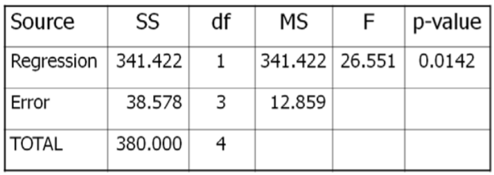
\(F=341.422 / 12.859=26.551\), que es más que el valor crítico de 10.13, por lo que Rechazar\(H_o\). Además, el\(p\) ‐valor = 0.0142 < 0.05 que también soporta rechazo\(H_o\).
Conclusión
Las ventas de Gafas de Sol y Lluvia están negativamente correlacionadas.