04. Aplicación de la segunda ley de Newton a un sistema de masa de resorte

1. Aplicación de la segunda ley de Newton a un sistema de masa de resorte

Aplicación de la segunda ley de Newton a un sistema de masa de resorte

Dado que no analizamos sistemas que involucran resortes en la sección dinámica anterior, deberíamos reponer esa omisión ahora.

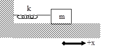
El sistema anterior consiste en un resorte con constante de resorte k unido a un bloque de masa m que descansa sobre una superficie sin fricción. El origen del sistema de coordenadas se ubica en la posición en la que el resorte está sin estirar.

Ahora imagina que el bloque se tira hacia la derecha y se suelta. Ojalá puedas convencerte de que el bloque oscilará de un lado a otro. Apliquemos la Segunda Ley de Newton en el instante en que la masa está en una posición arbitraria, x. La única fuerza que actúa sobre la masa en la dirección x es la fuerza del resorte.

\[ \sum \vec{F} = m\vec{a} \]

\[ \vec{F_{spring}} = m\vec{a} \]

\[ -ks =ma \]

Debido a nuestra elección del sistema de coordenadas, el estiramiento de los muelles es exactamente igual a la ubicación del bloque (x). Por lo tanto,

\[ -kx =ma \]

Tenga en cuenta que cuando el bloque está en una posición positibe, la fuerza del resorte está en la dirección negativa y cuando el bloque está en posiciones negativas, la fuerza del resorte está en la dirección positiva. Así, la fuerza del resorte siempre actúa para devolver el bloque al equilibrio.

Reorganizar da

y definiendo una constante, w ², como

(Concedido, parece bastante tonto definir ^k/_m como el cuadrado de una constante, pero solo seguir el juego. También te puede resultar frustrante saber que este “omega” no es una velocidad angular. ¡El bloque ni siquiera tiene una velocidad angular!)

rendimientos,

\[ -\omega^2 x=\dfrac{d^2x}{dt^2} \]

Por lo tanto, la función de posición para el bloque debe tener una derivada de segunda vez igual al producto de (- w ²) y a sí misma. Las únicas funciones cuya segunda derivada de tiempo es igual al producto de una constante negativa y en sí mismas ar las funciones seno y coseno. Por lo tanto, se puede escribir una solución a esta ecuación diferencial ¹:

\[ x(t) = A\;cos(\omega t+\phi)\]

or equivalently with the sine function, where A and \(\phi\) are arbitrary constants.²

• A is the amplitude of the oscillation. The amplitude is the maximum displacement of the object from equilibrium.
• \(\phi\) is the phase angle. The phase angle is used to adjust the function forward or backward in time. For example, if the particle is at the origin at t = 0 s, \(\phi\) must equal \(+\pi/2 \) or \(-\pi/2 \) to ensure that the cosine function evaluates to zero at t = 0 s. If the particle is at its maximum position at t = 0 s, then the phase angle must be zero or \(\pi\) to ensure that the cosine function evalutes to +1 or -1 at t = 0 s.
• \(\omega\) is the angular frequency of the oscillation.³

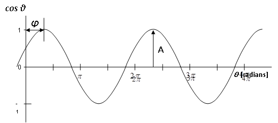
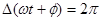
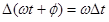
Note that the cosine function repeats itself when its argument increases by \(2\pi\). Thus, when

the function repeats. Since \(\omega\) and \(\phi\) are constant,

Therefore, the time interval when

is the time interval for one complete cycle of the oscillatory motion. The time for one complete cycle of the motion is termed the period, T. Thus,

Therefore, the physical significance of the angular frequency is that it is inversely proportional to the period.

Substituting in the definition of \(\omega\):

yields

In summary, a mass attached to a spring will oscillate about its equilibrium position with a position function given by:

This function repeats with a period of

---

1. A differential equation is an equation involving a function and its derivative(s).
2. To prove to yourself that this is indeed the solution to the equation, you should substitute the function, x(t), into the left side of the equation and the second derivative of x(t) into the right side. This will verify that the two sides of the equation are equal. In addition to mathematically verifying this solution, you should verify the solution physically by sketching a graph of the motion that youknow would result if the block were displaced to the right and comparing that sketch to a sketch of the function.
3. Again, note that \(\omega\)is not the angular velocity. The block is not rotating; it does not have an angular velocity.

Template:Paul