2.7: La ecuación de Schrödinger en dimensiones superiores

El análisis de pozos cuánticos y materiales a granel requiere que resolvamos la Ecuación de Schrödinger en 2-d y 3-d. La ecuación en 1-d

\[ \left[-\frac{\hbar^{2}}{2 m} \frac{d^{2}}{d x^{2}}+V(x)\right] \psi(x)=E \psi(x) \nonumber \]

se extiende a dimensiones más altas de la siguiente manera:

El operador de energía cinética

En 1-d

\[ \hat{T}=\frac{\hat{p}_{x}^{2}}{2m} \nonumber \]

Ahora, se puede escribir la magnitud del impulso en 3-d

\[ |\textbf{p}|^{2} = p_{x}^{2}+p_{y}^{2}+p_{z}^{2} \nonumber \]

Donde\(p_{x}\),\(p_{y}\) y\(p_{z}\) son los componentes del momentum en los ejes x, y y z, respectivamente. De ello se deduce que en 3-d

\[ \hat{T}=\frac{\hat{p}_{x}^{2}}{2m}+\frac{\hat{p}_{y}^{2}}{2m}+\dfrac{\hat{p}_{z}^{2}}{2m} = -\frac{\hbar^{2}}{2m}\left(\frac{d^{2}}{dx^{2}}+\frac{d^{2}}{dy^{2}}+\frac{d^{2}}{dz^{2}}\right) \nonumber \]

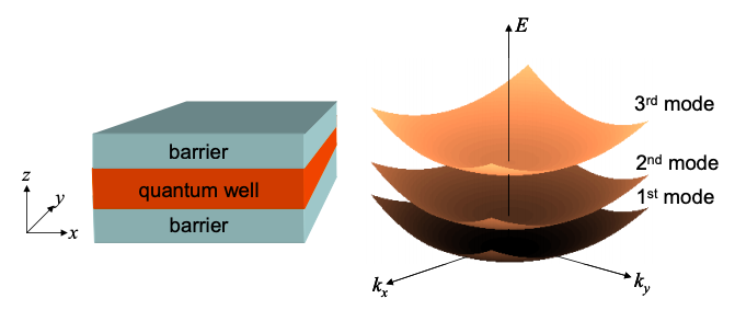
Potencial Separable — Pozo Cuántico

Un pozo cuántico se muestra en la Figura 2.6.2 (a). Supondremos que el potencial se puede separar en términos dependientes de x, y y z

\[ V(x,y,z)=V_{x}(x)+V_{y}(y)+V_{z}(z) \nonumber \]

Por ejemplo, un potencial de pozo cuántico viene dado por

\[ V_{x}(x) = 0 \nonumber \]

\( V_{y}(y) = 0 \)

\( V_{z}(z) = 0 \)

donde en la aproximación de pozo cuadrado infinito\(V_{0} \rightarrow \infty\), y u es la función de paso de unidad.

Para potenciales de esta forma se puede separar la Ecuación de Schrödinger:

\[ {\left[-\frac{\hbar^{2}}{2 m} \frac{d^{2}}{d x^{2}}+V_{x}(x)\right] \psi(x, y, z)+\left[-\frac{\hbar^{2}}{2 m} \frac{d^{2}}{d y^{2}}+V_{y}(y)\right] \psi(x, y, z)} +\left[-\frac{\hbar^{2}}{2 m} \frac{d^{2}}{d z^{2}}+V_{z}(z)\right] \psi(x, y, z)=\left(E_{x}+E_{y}+E_{z}\right) \psi(x, y, z) \nonumber \]

La función de onda también se puede separar

\[ \psi(x,y,z) = \psi_{x}(x)\psi_{y}(y)\psi_{z}(z) \nonumber \]

A partir de las ecuaciones 1.28.1 y 1.28.2, las soluciones al potencial infinito del pozo cuántico son

\[ \psi(x, y, z)=\psi_{x}(x) \psi_{y}(y) \psi_{z}(z)=\sqrt{\frac{2}{L}} \sin \left(n \frac{\pi z}{L}\right) \cdot \exp \left[i k_{x} x\right] \cdot \exp \left[i k_{y} y\right] \nonumber \]

con

\[ E =E_{x}+E_{y}+E_{z} = \frac{\hbar^{2}k_{x}^{2}}{2m}+\frac{\hbar^{2}k_{y}^{2}}{2m}+\frac{n^{2}\hbar^{2}\pi^{2}}{2mL^{2}} \nonumber \]

Esta relación de dispersión se muestra en la Figura 2.7.1 para los tres modos más bajos del pozo cuántico.

Figura\(\PageIndex{1}\):. Un pozo cuántico confina electrones en 1 dimensión.

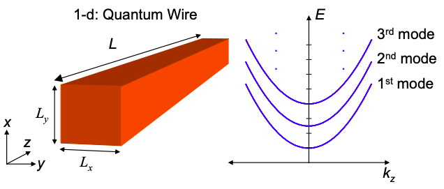
Potencial separable — Quantum Wire

En la Figura 2.6.2 (b) se muestra un alambre cuántico con sección transversal rectangular. Nuevamente, asumiremos que el potencial es infinito en los límites del cable:

\[ V(x,y,z) = V_{0}u(-x)+V_{0}u(x-L_{x})+V_{0}u(-y)+V_{0}u(x-L_{y}) \nonumber \]

donde\(V_{0} \rightarrow \infty\). La función de onda asociada está confinada en el plano x-y y compuesta por ondas planas en la dirección z, por lo que elegimos la función de onda de prueba

\[ \psi(x,y,z) = \psi(x,y)e^{ik_{z}z} \nonumber \]

Al insertar la ecuación 2.7.12 en la ecuación de Schrödinger se obtiene (for\(0 \leq x \leq L_{x}\) y\(0 \leq y \leq L_{y}\)):

\[ -\frac{\hbar^{2}}{2 m} \frac{d^{2}}{d x^{2}} \psi(x, y)-\frac{\hbar^{2}}{2 m} \frac{d^{2}}{d y^{2}} \psi(x, y)+\frac{\hbar^{2} k_{z}^{2}}{2 m} \psi(x, y)=E \psi(x, y) \nonumber \]

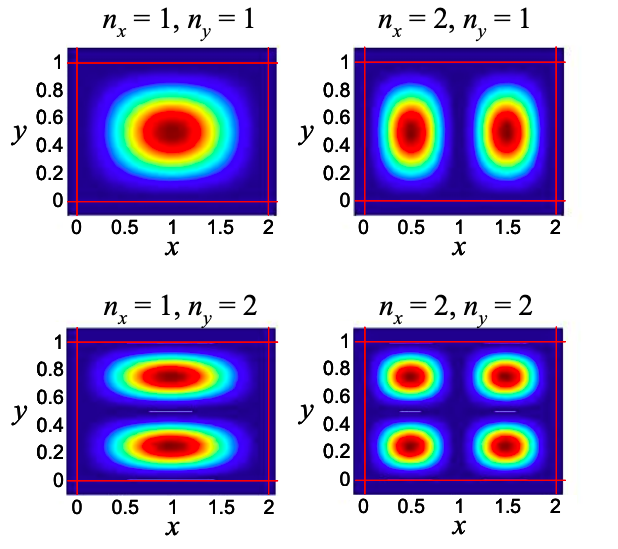
Dado que el potencial va al infinito en los bordes del cable,\(\psi(x=0)=\psi(x=L_{x})=\psi(y=0)=\psi(y=L_{y})\). Así, la solución es

\[ \psi(x,y)=\psi_{0}\sin(k_{x}x)\sin(k_{y}y), \nonumber \]

donde

\[ k_{x}=\frac{n_{x}\pi}{L_{x}},\ n_{x}=1,2,…,\ k_{y}=1,2,… \nonumber \]

Figura\(\PageIndex{2}\): Los primeros cuatro modos del cable cuántico. Ya que en este ejemplo,\(L_{x}>L_{y}\) el\(n_{x}=2,\ n_{y}=1\) modo tiene menor energía que el modo\ (n_ {x} =1,\ n_ {y} =2).

Así, la restricción en las direcciones x e y define los niveles de energía discretos

\[ E_{n_{x}, n_{y}}=\frac{\hbar^{2} \pi^{2}}{2 m}\left(\frac{n_{x}^{2}}{L_{x}^{2}}+\frac{n_{y}^{2}}{L_{y}^{2}}\right), \quad n_{x}, n_{y}=1,2, \ldots \nonumber \]

La energía total es

\[ E_{n_{x}, n_{y}}=\frac{\hbar^{2} \pi^{2}}{2 m}\left(\frac{n_{x}^{2}}{L_{x}^{2}}+\frac{n_{y}^{2}}{L_{y}^{2}}\right) + \frac{\hbar^{2}k_{z}^{2}}{2m}, \quad n_{x}, n_{y}=1,2, \ldots \nonumber \]

Esta relación de dispersión se representa en la Figura 2.7.3 para los tres modos más bajos.

Figura\(\PageIndex{3}\): Un cable cuántico confina electrones en 2 dimensiones.