8.2: Las relaciones trigonométricas

Última actualización
Guardar como PDF

Page ID: 111969

$ \newcommand{\vecs}[1]{\overset { \scriptstyle \rightharpoonup} {\mathbf{#1}} } $

$ \newcommand{\vecd}[1]{\overset{-\!-\!\rightharpoonup}{\vphantom{a}\smash {#1}}} $

$ \newcommand{\id}{\mathrm{id}}$ $ \newcommand{\Span}{\mathrm{span}}$

( \newcommand{\kernel}{\mathrm{null}\,}\) $ \newcommand{\range}{\mathrm{range}\,}$

$ \newcommand{\RealPart}{\mathrm{Re}}$ $ \newcommand{\ImaginaryPart}{\mathrm{Im}}$

$ \newcommand{\Argument}{\mathrm{Arg}}$ $ \newcommand{\norm}[1]{\| #1 \|}$

$ \newcommand{\inner}[2]{\langle #1, #2 \rangle}$

$ \newcommand{\Span}{\mathrm{span}}$

$ \newcommand{\id}{\mathrm{id}}$

$ \newcommand{\Span}{\mathrm{span}}$

$ \newcommand{\kernel}{\mathrm{null}\,}$

$ \newcommand{\range}{\mathrm{range}\,}$

$ \newcommand{\RealPart}{\mathrm{Re}}$

$ \newcommand{\ImaginaryPart}{\mathrm{Im}}$

$ \newcommand{\Argument}{\mathrm{Arg}}$

$ \newcommand{\norm}[1]{\| #1 \|}$

$ \newcommand{\inner}[2]{\langle #1, #2 \rangle}$

$ \newcommand{\Span}{\mathrm{span}}$ $ \newcommand{\AA}{\unicode[.8,0]{x212B}}$

$ \newcommand{\vectorA}[1]{\vec{#1}} % arrow$

$ \newcommand{\vectorAt}[1]{\vec{\text{#1}}} % arrow$

$ \newcommand{\vectorB}[1]{\overset { \scriptstyle \rightharpoonup} {\mathbf{#1}} } $

$ \newcommand{\vectorC}[1]{\textbf{#1}} $

$ \newcommand{\vectorD}[1]{\overrightarrow{#1}} $

$ \newcommand{\vectorDt}[1]{\overrightarrow{\text{#1}}} $

$ \newcommand{\vectE}[1]{\overset{-\!-\!\rightharpoonup}{\vphantom{a}\smash{\mathbf {#1}}}} $

$ \newcommand{\vecs}[1]{\overset { \scriptstyle \rightharpoonup} {\mathbf{#1}} } $

$ \newcommand{\vecd}[1]{\overset{-\!-\!\rightharpoonup}{\vphantom{a}\smash {#1}}} $

$\newcommand{\avec}{\mathbf a}$ $\newcommand{\bvec}{\mathbf b}$ $\newcommand{\cvec}{\mathbf c}$ $\newcommand{\dvec}{\mathbf d}$ $\newcommand{\dtil}{\widetilde{\mathbf d}}$ $\newcommand{\evec}{\mathbf e}$ $\newcommand{\fvec}{\mathbf f}$ $\newcommand{\nvec}{\mathbf n}$ $\newcommand{\pvec}{\mathbf p}$ $\newcommand{\qvec}{\mathbf q}$ $\newcommand{\svec}{\mathbf s}$ $\newcommand{\tvec}{\mathbf t}$ $\newcommand{\uvec}{\mathbf u}$ $\newcommand{\vvec}{\mathbf v}$ $\newcommand{\wvec}{\mathbf w}$ $\newcommand{\xvec}{\mathbf x}$ $\newcommand{\yvec}{\mathbf y}$ $\newcommand{\zvec}{\mathbf z}$ $\newcommand{\rvec}{\mathbf r}$ $\newcommand{\mvec}{\mathbf m}$ $\newcommand{\zerovec}{\mathbf 0}$ $\newcommand{\onevec}{\mathbf 1}$ $\newcommand{\real}{\mathbb R}$ $\newcommand{\twovec}[2]{\left[\begin{array}{r}#1 \\ #2 \end{array}\right]}$ $\newcommand{\ctwovec}[2]{\left[\begin{array}{c}#1 \\ #2 \end{array}\right]}$ $\newcommand{\threevec}[3]{\left[\begin{array}{r}#1 \\ #2 \\ #3 \end{array}\right]}$ $\newcommand{\cthreevec}[3]{\left[\begin{array}{c}#1 \\ #2 \\ #3 \end{array}\right]}$ $\newcommand{\fourvec}[4]{\left[\begin{array}{r}#1 \\ #2 \\ #3 \\ #4 \end{array}\right]}$ $\newcommand{\cfourvec}[4]{\left[\begin{array}{c}#1 \\ #2 \\ #3 \\ #4 \end{array}\right]}$ $\newcommand{\fivevec}[5]{\left[\begin{array}{r}#1 \\ #2 \\ #3 \\ #4 \\ #5 \\ \end{array}\right]}$ $\newcommand{\cfivevec}[5]{\left[\begin{array}{c}#1 \\ #2 \\ #3 \\ #4 \\ #5 \\ \end{array}\right]}$ $\newcommand{\mattwo}[4]{\left[\begin{array}{rr}#1 \amp #2 \\ #3 \amp #4 \\ \end{array}\right]}$ $\newcommand{\laspan}[1]{\text{Span}\{#1\}}$ $\newcommand{\bcal}{\cal B}$ $\newcommand{\ccal}{\cal C}$ $\newcommand{\scal}{\cal S}$ $\newcommand{\wcal}{\cal W}$ $\newcommand{\ecal}{\cal E}$ $\newcommand{\coords}[2]{\left\{#1\right\}_{#2}}$ $\newcommand{\gray}[1]{\color{gray}{#1}}$ $\newcommand{\lgray}[1]{\color{lightgray}{#1}}$ $\newcommand{\rank}{\operatorname{rank}}$ $\newcommand{\row}{\text{Row}}$ $\newcommand{\col}{\text{Col}}$ $\renewcommand{\row}{\text{Row}}$ $\newcommand{\nul}{\text{Nul}}$ $\newcommand{\var}{\text{Var}}$ $\newcommand{\corr}{\text{corr}}$ $\newcommand{\len}[1]{\left|#1\right|}$ $\newcommand{\bbar}{\overline{\bvec}}$ $\newcommand{\bhat}{\widehat{\bvec}}$ $\newcommand{\bperp}{\bvec^\perp}$ $\newcommand{\xhat}{\widehat{\xvec}}$ $\newcommand{\vhat}{\widehat{\vvec}}$ $\newcommand{\uhat}{\widehat{\uvec}}$ $\newcommand{\what}{\widehat{\wvec}}$ $\newcommand{\Sighat}{\widehat{\Sigma}}$ $\newcommand{\lt}{<}$ $\newcommand{\gt}{>}$ $\newcommand{\amp}{&}$ $\definecolor{fillinmathshade}{gray}{0.9}$

Hay seis relaciones trigonométricas comunes que relacionan los lados de un triángulo rectángulo con los ángulos dentro del triángulo. Las tres relaciones estándar son el seno, el coseno y la tangente. Estos suelen abreviarse pecado, cos y bronceado. Los otros tres (cosecante, secante y cotangente) son los recíprocos del seno, coseno y tangente y a menudo se abrevian csc, sec y cot.

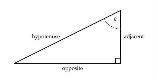
$clipboard_e1e671f5fb827aa8e16ea323dd1bf79cf.png$

Dado un ángulo situado en un triángulo rectángulo, la función sinusoidal se define como la relación del lado opuesto al ángulo a la hipotenusa, el coseno se define como la relación del lado adyacente al ángulo a la hipotenusa y la tangente se define como la relación del lado opuesto al ángulo al lado adyacente al ángulo.
\ [ \ begin {aligned}
\ sin\ theta &=\ frac {o p p} {h y p}\\
\ cos\ theta &=\ frac {a d j} {h y p}\\
\ tan\ theta &=\ frac {o p p} {a d j}
\ end {alineado}
\] Un dispositivo monumónico común para ayudar a recordar estos relaciones es
-Sohcahtoa-que identifica el pecado como Opp sobre Hyp Cos como Adj sobre Hyp y el Tan como Opp sobre Adj.

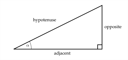
Un ángulo agudo colocado en la otra posición de un triángulo rectángulo tendría diferentes lados oppositos y adyacentes aunque la hipotenusa permanecería igual.

$clipboard_e49ef8fdb73380a1430c79aac039b0abb.png$

Ejemplos: Ratios trigonométricos
Encontrar$\sin \theta, \cos \theta$ y$\tan \theta$ para el ángulo$\theta$

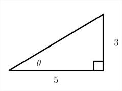
$clipboard_efb73cc1b837f654a6d62b99388a47ce2.png$

dado Para encontrar el pecado y cos del ángulo$\theta$, primero debemos encontrar la hipotenusa usando el Teorema de Pitágoras $\left(a^{2}+b^{2}=c^{2}\right)$

ya que conocemos las patas del triángulo, podemos sustituir estos valores por$a$ y$b$ en el Teorema de Pitágoras:
\ [ \ begin {array} {c}
3^ {2} +5^ {2} =c^ {2}\\
9+25=c^ {2}\\
34=c^ {2}\
\ sqrt {34} =c
\ end {array }
\] Ahora que conocemos la hipotenusa$(\sqrt{34}),$ podemos determinar el pecado, cos y bronceado para el ángulo$\theta$
\ [ \ begin {alineado}
\ sin\ theta &=\ frac {3} {\ sqrt {34}}\\
\ cos\ theta &=\ frac {5} {\ sqrt {34}}\\
\ tan\ theta &=\ frac {3} {5}
\ end {alineado}
\] Buscar$\sin \theta, \cos \theta$ y$\tan \theta$ para el ángulo dado$\theta$

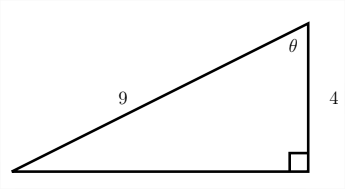
$clipboard_ea2d08b3e66d666076689a39e4381a25f.png$

Nuevamente, para encontrar el pecado, cos y tan del ángulo$\theta,$ debemos encontrar el lado faltante del triángulo usando el Teoreoreas de Pitágoras. ya que, en este caso, conocemos la hipotenusa y una de las piernas, se debe sustituir el valor de la hipotenusa$c$ y la longitud de la pierna estamos dado puede ser sustituido por cualquiera
$a$ o$b$

\ [ \ begin {array} {c}
4^ {2} +b^ {2} =9^ {2}\\
16+b^ {2} =81\\
b^ {2} =65\\
b=\ sqrt {65}
\ end {array}
\] Ahora que conocemos la longitud de la otra pata del triángulo$(\sqrt{65}),$ podemos determinar el pecado, cos y para el bronceado angle$\theta$
\ [ \ begin {aligned}
\ sin\ theta &=\ frac {\ sqrt {65}} {9}\
\\ cos\ theta &=\ frac {4} {9}\
\\ tan\ theta &=\ frac {\ sqrt {65}} {4}
\ end {alineado}
\] Además de los ejemplos anteriores, si estamos dado el valor de una de las relaciones trigonométricas, podemos encontrar el valor de las otras dos.
Ejemplo
Dado que$\cos \theta=\frac{1}{3},$ encontrar$\sin \theta$ y$\tan \theta$
Dada la información sobre el coseno del ángulo$\theta,$ podemos crear un triángulo que nos permitirá encontrar$\sin \theta$ y$\tan \theta$

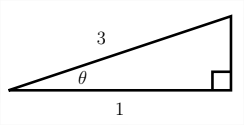
$clipboard_e4e14eb1e316d6a490de49b3b565009d9.png$

Usando el Teorema de Pitágoras, podemos encontrar el lado faltante del triángulo:
\ [ \ begin {array} {c}
a^ {2} +1^ {2} =3^ {2}\\
a^ {2} +1=9
\ end {array}
\] $a^{2}=8$
$a=\sqrt{8}=2 \sqrt{2}$
Entonces$\sin \theta=\frac{\sqrt{8}}{3}$ y$\tan \theta=\frac{\sqrt{8}}{1}=\sqrt{8}$
Podrías decirte a ti mismo: “Espera un minuto, solo porque el coseno del ángulo$\theta$ es$\frac{1}{3},$ eso no significa necesariamente que los lados del triángulo sean 1 y$3,$ podrían ser 2 y$6,$ o 3 y 9 o cualquier valor$n$ y$3 n . "$

Esto es cierto, y si los lados se expresan como$n$ y$3 n,$ entonces el lado faltante sería$n \sqrt{8},$ para que cada vez que encontremos una relación trigonométrica, el$n^{\prime}$ s se cancelará, así que simplemente los dejamos afuera para empezar y llamar a los lados 1 y 3
Ejemplo
Dado ese$\tan \theta=\frac{\sqrt{5}}{7},$ hallazgo$\sin \theta$ y$\cos \theta$
Primero tomaremos la información sobre la tangente y usaremos esta para dibujar un triángulo.

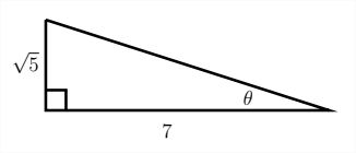
$clipboard_e8cc70b82d0976667be71e5e4b87a97f2.png$

Luego usa el Teorema de Pitágoras para encontrar el lado faltante del triángulo:
\ [\ begin {array} {c}
\ sqrt {5} ^ {2} +7^ {2} =c^ {2}\\
5+49=c^ {2}\\
54=c^ {2}
\\ sqrt {54} =3\ sqrt {6} =c
\ end {array}
\] Entonces:
\ [ \ sin\ theta=\ frac {\ sqrt {5}} {\ sqrt {54}} =\ sqrt {\ frac {5} {54}}
\] \ [ \ cos\ theta=\ frac {7} {\ sqrt {54}} =\ frac {7} {3\ sqrt {6}}
\]

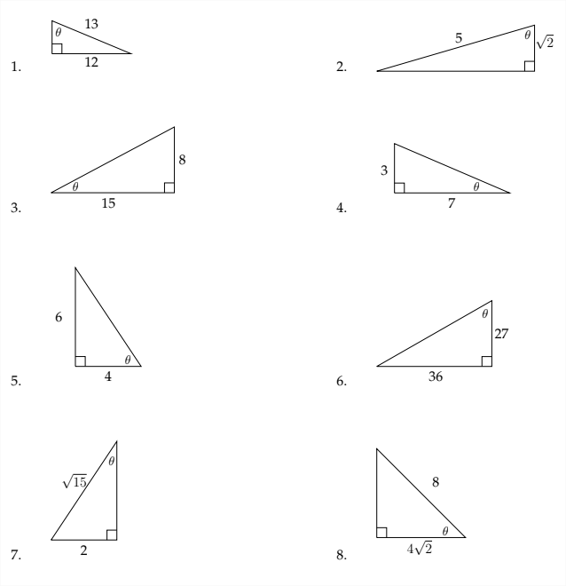
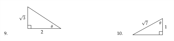
Ejercicios 1.2
Encontrar$\sin \theta, \cos \theta$ y$\tan \theta$ para los triángulos dados.

$clipboard_e84ab3159821579e9c33b8ee835c05230.png$

$clipboard_e6b7e7492045195da2d332ba850f2165c.png$

Utilice la información proporcionada para encontrar las otras dos relaciones trigonométricas.
11. $\quad \tan \theta=\frac{1}{2}$
12. $\quad \sin \theta=\frac{3}{4}$
13. $\quad \cos \theta=\frac{3}{\sqrt{20}}$
14. $\quad \tan \theta=2$
15. $\sin \theta=\frac{5}{\sqrt{40}}$
16. $\sin \theta=\frac{7}{10}$
17. $\cos \theta=\frac{9}{40}$
18. $\quad \tan \theta=\sqrt{3}$
19. $\cos \theta=\frac{1}{2}$
20. $\cos \theta=\frac{3}{7}$
21. $\sin \theta=\frac{\sqrt{5}}{7}$
22. $\quad \tan \theta=1.5$

Search

Text Color

Text Size

Margin Size

Font Type