6.3: Inhibición Competitiva
- Page ID
- 117632

\( \newcommand{\vecs}[1]{\overset { \scriptstyle \rightharpoonup} {\mathbf{#1}} } \)
\( \newcommand{\vecd}[1]{\overset{-\!-\!\rightharpoonup}{\vphantom{a}\smash {#1}}} \)
\( \newcommand{\dsum}{\displaystyle\sum\limits} \)
\( \newcommand{\dint}{\displaystyle\int\limits} \)
\( \newcommand{\dlim}{\displaystyle\lim\limits} \)
\( \newcommand{\id}{\mathrm{id}}\) \( \newcommand{\Span}{\mathrm{span}}\)
( \newcommand{\kernel}{\mathrm{null}\,}\) \( \newcommand{\range}{\mathrm{range}\,}\)
\( \newcommand{\RealPart}{\mathrm{Re}}\) \( \newcommand{\ImaginaryPart}{\mathrm{Im}}\)
\( \newcommand{\Argument}{\mathrm{Arg}}\) \( \newcommand{\norm}[1]{\| #1 \|}\)
\( \newcommand{\inner}[2]{\langle #1, #2 \rangle}\)
\( \newcommand{\Span}{\mathrm{span}}\)
\( \newcommand{\id}{\mathrm{id}}\)
\( \newcommand{\Span}{\mathrm{span}}\)
\( \newcommand{\kernel}{\mathrm{null}\,}\)
\( \newcommand{\range}{\mathrm{range}\,}\)
\( \newcommand{\RealPart}{\mathrm{Re}}\)
\( \newcommand{\ImaginaryPart}{\mathrm{Im}}\)
\( \newcommand{\Argument}{\mathrm{Arg}}\)
\( \newcommand{\norm}[1]{\| #1 \|}\)
\( \newcommand{\inner}[2]{\langle #1, #2 \rangle}\)
\( \newcommand{\Span}{\mathrm{span}}\) \( \newcommand{\AA}{\unicode[.8,0]{x212B}}\)
\( \newcommand{\vectorA}[1]{\vec{#1}} % arrow\)
\( \newcommand{\vectorAt}[1]{\vec{\text{#1}}} % arrow\)
\( \newcommand{\vectorB}[1]{\overset { \scriptstyle \rightharpoonup} {\mathbf{#1}} } \)
\( \newcommand{\vectorC}[1]{\textbf{#1}} \)
\( \newcommand{\vectorD}[1]{\overrightarrow{#1}} \)
\( \newcommand{\vectorDt}[1]{\overrightarrow{\text{#1}}} \)
\( \newcommand{\vectE}[1]{\overset{-\!-\!\rightharpoonup}{\vphantom{a}\smash{\mathbf {#1}}}} \)
\( \newcommand{\vecs}[1]{\overset { \scriptstyle \rightharpoonup} {\mathbf{#1}} } \)
\(\newcommand{\longvect}{\overrightarrow}\)
\( \newcommand{\vecd}[1]{\overset{-\!-\!\rightharpoonup}{\vphantom{a}\smash {#1}}} \)
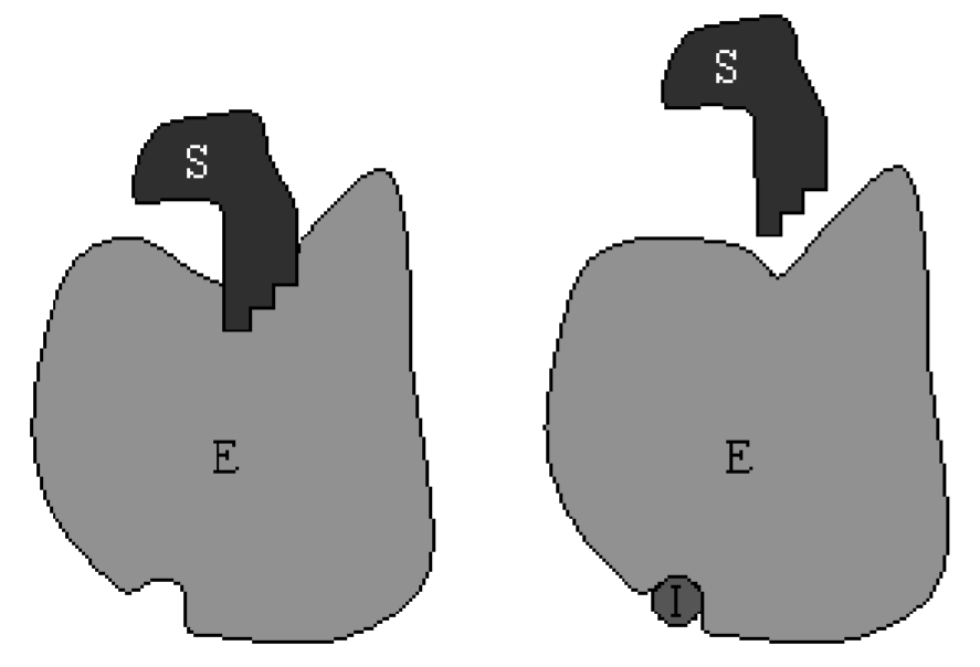
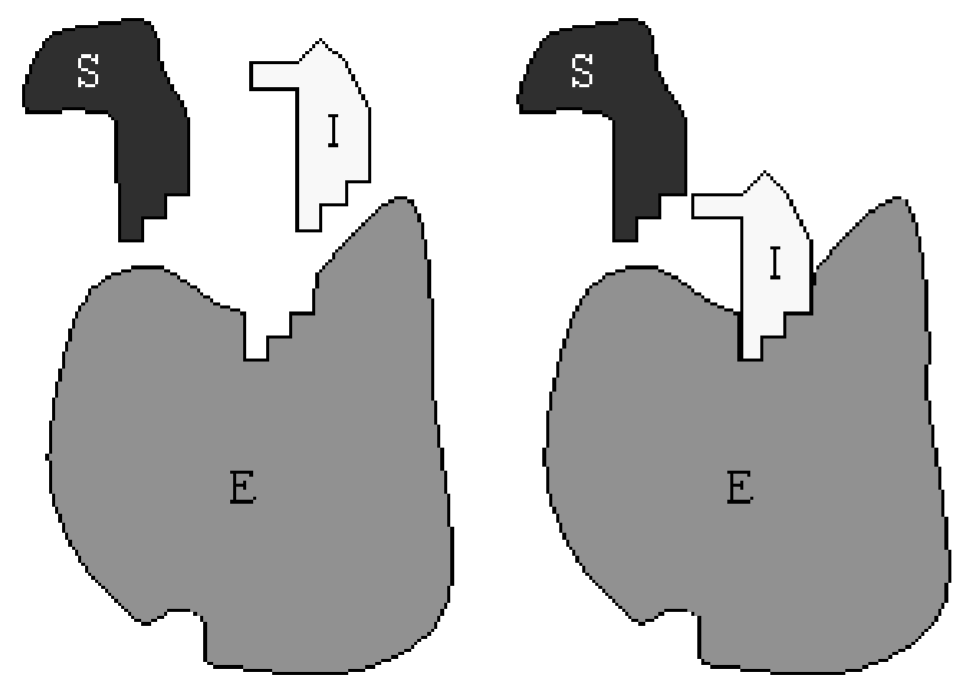
\(\newcommand{\avec}{\mathbf a}\) \(\newcommand{\bvec}{\mathbf b}\) \(\newcommand{\cvec}{\mathbf c}\) \(\newcommand{\dvec}{\mathbf d}\) \(\newcommand{\dtil}{\widetilde{\mathbf d}}\) \(\newcommand{\evec}{\mathbf e}\) \(\newcommand{\fvec}{\mathbf f}\) \(\newcommand{\nvec}{\mathbf n}\) \(\newcommand{\pvec}{\mathbf p}\) \(\newcommand{\qvec}{\mathbf q}\) \(\newcommand{\svec}{\mathbf s}\) \(\newcommand{\tvec}{\mathbf t}\) \(\newcommand{\uvec}{\mathbf u}\) \(\newcommand{\vvec}{\mathbf v}\) \(\newcommand{\wvec}{\mathbf w}\) \(\newcommand{\xvec}{\mathbf x}\) \(\newcommand{\yvec}{\mathbf y}\) \(\newcommand{\zvec}{\mathbf z}\) \(\newcommand{\rvec}{\mathbf r}\) \(\newcommand{\mvec}{\mathbf m}\) \(\newcommand{\zerovec}{\mathbf 0}\) \(\newcommand{\onevec}{\mathbf 1}\) \(\newcommand{\real}{\mathbb R}\) \(\newcommand{\twovec}[2]{\left[\begin{array}{r}#1 \\ #2 \end{array}\right]}\) \(\newcommand{\ctwovec}[2]{\left[\begin{array}{c}#1 \\ #2 \end{array}\right]}\) \(\newcommand{\threevec}[3]{\left[\begin{array}{r}#1 \\ #2 \\ #3 \end{array}\right]}\) \(\newcommand{\cthreevec}[3]{\left[\begin{array}{c}#1 \\ #2 \\ #3 \end{array}\right]}\) \(\newcommand{\fourvec}[4]{\left[\begin{array}{r}#1 \\ #2 \\ #3 \\ #4 \end{array}\right]}\) \(\newcommand{\cfourvec}[4]{\left[\begin{array}{c}#1 \\ #2 \\ #3 \\ #4 \end{array}\right]}\) \(\newcommand{\fivevec}[5]{\left[\begin{array}{r}#1 \\ #2 \\ #3 \\ #4 \\ #5 \\ \end{array}\right]}\) \(\newcommand{\cfivevec}[5]{\left[\begin{array}{c}#1 \\ #2 \\ #3 \\ #4 \\ #5 \\ \end{array}\right]}\) \(\newcommand{\mattwo}[4]{\left[\begin{array}{rr}#1 \amp #2 \\ #3 \amp #4 \\ \end{array}\right]}\) \(\newcommand{\laspan}[1]{\text{Span}\{#1\}}\) \(\newcommand{\bcal}{\cal B}\) \(\newcommand{\ccal}{\cal C}\) \(\newcommand{\scal}{\cal S}\) \(\newcommand{\wcal}{\cal W}\) \(\newcommand{\ecal}{\cal E}\) \(\newcommand{\coords}[2]{\left\{#1\right\}_{#2}}\) \(\newcommand{\gray}[1]{\color{gray}{#1}}\) \(\newcommand{\lgray}[1]{\color{lightgray}{#1}}\) \(\newcommand{\rank}{\operatorname{rank}}\) \(\newcommand{\row}{\text{Row}}\) \(\newcommand{\col}{\text{Col}}\) \(\renewcommand{\row}{\text{Row}}\) \(\newcommand{\nul}{\text{Nul}}\) \(\newcommand{\var}{\text{Var}}\) \(\newcommand{\corr}{\text{corr}}\) \(\newcommand{\len}[1]{\left|#1\right|}\) \(\newcommand{\bbar}{\overline{\bvec}}\) \(\newcommand{\bhat}{\widehat{\bvec}}\) \(\newcommand{\bperp}{\bvec^\perp}\) \(\newcommand{\xhat}{\widehat{\xvec}}\) \(\newcommand{\vhat}{\widehat{\vvec}}\) \(\newcommand{\uhat}{\widehat{\uvec}}\) \(\newcommand{\what}{\widehat{\wvec}}\) \(\newcommand{\Sighat}{\widehat{\Sigma}}\) \(\newcommand{\lt}{<}\) \(\newcommand{\gt}{>}\) \(\newcommand{\amp}{&}\) \(\definecolor{fillinmathshade}{gray}{0.9}\)La inhibición competitiva ocurre cuando las moléculas inhibidorascompiten con las moléculas de sustrato para unirse al sitio activode la misma enzima. Cuando un inhibidor está unido a la enzima, no se produce ningún producto por lo que la inhibición competitiva reducirá la velocidad de la reacción. Una caricatura de este proceso se muestra en la Fig. \(6.2\).
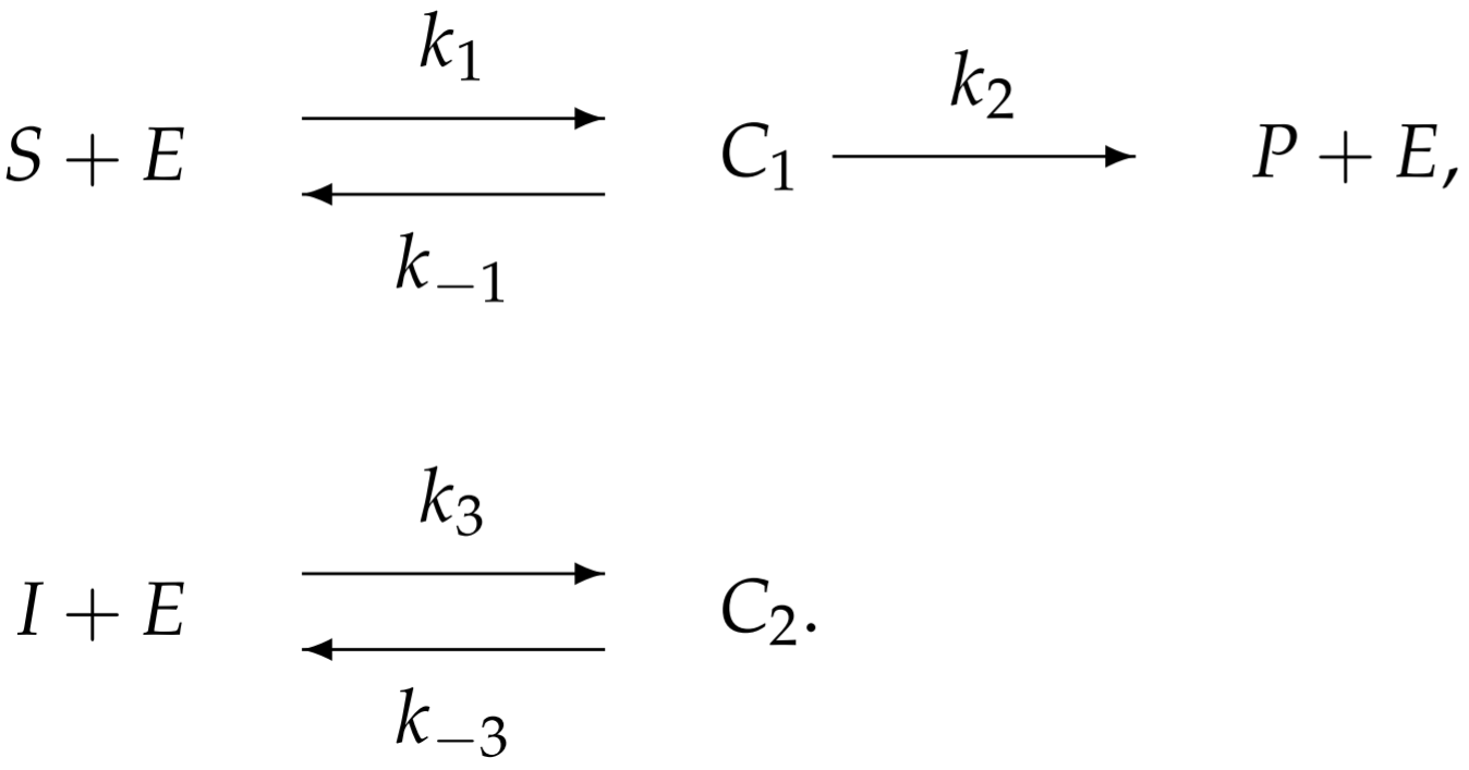
Para modelar la inhibición competitiva, se introduce una reacción adicional asociada con la unión inhibidor-enzima:
Con reacciones enzimáticas más complicadas, el esquema de reacción se vuelve difícil de interpretar. Quizás una manera más fácil de visualizar la reacción es a partir del siguiente esquema redibujado:
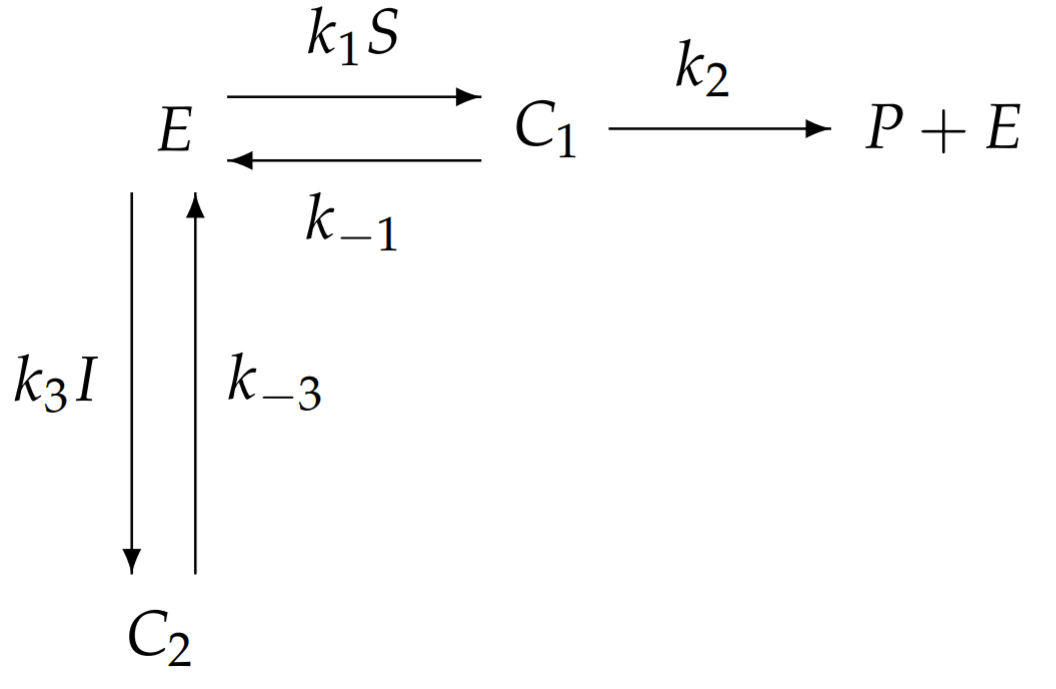
Aquí, el sustrato\(S\) y el inhibidor\(I\) se combinan con las constantes de velocidad relevantes, en lugar de tratarse por separado. Es inmediatamente obvio a partir de este esquema redibujado que la inhibición se logra secuestrando la enzima en forma de\(C_{2}\) e impidiendo su participación en la catálisis de\(S\) a\(P\).
Nuestro objetivo es determinar la velocidad de reacción\(\dot{P}\) en términos de las concentraciones de sustrato e inhibidor, y la concentración total de la enzima (libre y unida). La ley de acción masiva aplicada a los dos complejos y el producto da como resultado
\[\begin{aligned} \frac{d C_{1}}{d t} &=k_{1} S E-\left(k_{-1}+k_{2}\right) C_{1} \\[4pt] \frac{d C_{2}}{d t} &=k_{3} I E-k_{-3} C_{2} \\[4pt] \frac{d P}{d t} &=k_{2} C_{1} \end{aligned} \nonumber \]
La enzima, libre y unida, se conserva para que
\[\frac{d}{d t}\left(E+C_{1}+C_{2}\right)=0 \quad \Longrightarrow \quad E+C_{1}+C_{2}=E_{0} \quad \Longrightarrow \quad E=E_{0}-C_{1}-C_{2} . \nonumber \]
Bajo la aproximación cuasi-equilibrio,\(C_{1}=\dot{C}_{2}=0\), de modo que
\[\begin{array}{r} k_{1} S\left(E_{0}-C_{1}-C_{2}\right)-\left(k_{-1}+k_{2}\right) C_{1}=0, \\[4pt] k_{3} I\left(E_{0}-C_{1}-C_{2}\right)-k_{-3} C_{2}=0, \end{array} \nonumber \]
lo que da como resultado el siguiente sistema de dos ecuaciones lineales y dos incógnitas\(\left(C_{1}\right.\) y\(\left.C_{2}\right)\):
\[\begin{align} \left(k_{-1}+k_{2}+k_{1} S\right) C_{1}+k_{1} S C_{2} &=k_{1} E_{0} S \\[4pt] k_{3} I C_{1}+\left(k_{-3}+k_{3} I\right) C_{2} &=k_{3} E_{0} I \end{align} \nonumber \]
Definimos la constante de Michaelis-Menten\(K_{m}\) como antes, y una constante adicional\(K_{i}\) asociada con la reacción inhibidora:
\[K_{m}=\frac{k_{-1}+k_{2}}{k_{1}}, \quad K_{i}=\frac{k_{-3}}{k_{3}} \nonumber \]
Dividir\((6.3.2)\) por\(k_{1}\) y\((6.3.3)\) por\(k_{3}\) rendimientos
\[\begin{align} \left(K_{m}+S\right) C_{1}+S C_{2} &=E_{0} S \\[4pt] I C_{1}+\left(K_{i}+I\right) C_{2} &=E_{0} I \end{align} \nonumber \]
Dado que nuestro objetivo es obtener la velocidad de la reacción, que requiere determinar\(C_{1}\), multiplicamos\((6.3.5)\) por\(\left(K_{i}+I\right)\) y\((6.3.6)\) por\(S\), y restamos:
\[\begin{aligned} \left(K_{m}+S\right)\left(K_{i}+I\right) C_{1}+S\left(K_{i}+I\right) C_{2} &=E_{0}\left(K_{i}+I\right) S \\[4pt] S I C_{1}+S\left(K_{i}+I\right) C_{2} &=E_{0} S I \\[4pt] \left(\left(K_{m}+S\right)\left(K_{i}+I\right)-S I\right) C_{1} &=K_{i} E_{0} S \end{aligned} \nonumber \]
o después de la cancelación y reorganización
\[\begin{aligned} C_{1} &=\frac{K_{i} E_{0} S}{K_{m} K_{i}+K_{i} S+K_{m} I} \\[4pt] &=\frac{E_{0} S}{K_{m}\left(1+I / K_{i}\right)+S} \end{aligned} \nonumber \]
Por lo tanto, la velocidad de reacción viene dada por
\[\begin{align} \frac{d P}{d t} &=\frac{\left(k_{2} E_{0}\right) S}{K_{m}\left(1+I / K_{i}\right)+S} \nonumber \\[4pt] &=\frac{V_{m} S}{K_{m}^{\prime}+S} \end{align} \nonumber \]
donde
\[V_{m}=k_{2} E_{0}, \quad K_{m}^{\prime}=K_{m}\left(1+I / K_{i}\right) . \nonumber \]
Al comparar la velocidad de reacción inhibida\((6.3.7)\) y\((6.3.8)\) con la velocidad de reacción desinhibida\((6.2.6)\) y\((6.2.7)\), observamos que la inhibición aumenta la constante de Michaelis-Menten de la reacción, pero deja sin cambios la reacción máxima velocidad. Dado que la constante de Michaelis-Menten se define como la concentración de sustrato requerida para alcanzar la mitad de la velocidad máxima de reacción, la adición de un inhibidor con una concentración de sustrato fija actúa para disminuir la velocidad de reacción. Sin embargo, una reacción saturada con sustrato aún alcanza la velocidad de reacción máxima desinhibida.