5.5: Proyección Fisher

Última actualización
Guardar como PDF

Page ID: 76479

\( \newcommand{\vecs}[1]{\overset { \scriptstyle \rightharpoonup} {\mathbf{#1}} } \) \( \newcommand{\vecd}[1]{\overset{-\!-\!\rightharpoonup}{\vphantom{a}\smash {#1}}} \)\(\newcommand{\id}{\mathrm{id}}\) \( \newcommand{\Span}{\mathrm{span}}\) \( \newcommand{\kernel}{\mathrm{null}\,}\) \( \newcommand{\range}{\mathrm{range}\,}\) \( \newcommand{\RealPart}{\mathrm{Re}}\) \( \newcommand{\ImaginaryPart}{\mathrm{Im}}\) \( \newcommand{\Argument}{\mathrm{Arg}}\) \( \newcommand{\norm}[1]{\| #1 \|}\) \( \newcommand{\inner}[2]{\langle #1, #2 \rangle}\) \( \newcommand{\Span}{\mathrm{span}}\) \(\newcommand{\id}{\mathrm{id}}\) \( \newcommand{\Span}{\mathrm{span}}\) \( \newcommand{\kernel}{\mathrm{null}\,}\) \( \newcommand{\range}{\mathrm{range}\,}\) \( \newcommand{\RealPart}{\mathrm{Re}}\) \( \newcommand{\ImaginaryPart}{\mathrm{Im}}\) \( \newcommand{\Argument}{\mathrm{Arg}}\) \( \newcommand{\norm}[1]{\| #1 \|}\) \( \newcommand{\inner}[2]{\langle #1, #2 \rangle}\) \( \newcommand{\Span}{\mathrm{span}}\)\(\newcommand{\AA}{\unicode[.8,0]{x212B}}\)

Para las discusiones hasta el momento, se ha utilizado la fórmula de perspectiva con cuñas sólidas y discontinuas para representar la disposición 3D de grupos unidos a un centro de quiralidad. Aparte de eso, hay otra fórmula ampliamente aplicada para ese propósito, es decir, la proyección Fisher. Una proyección Fisher es un atajo para mostrar la disposición de grupos espaciales de un centro de quiralidad, es más fácil de dibujar y reconocer, y es particularmente útil para mostrar las estructuras con más de un centro de quiralidad.

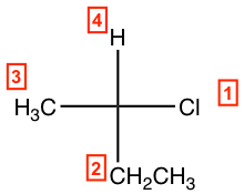
En la proyección Fisher, el centro de quiralidad se muestra como la intersección de dos líneas perpendiculares. Las líneas horizontales representan los enlaces que apuntan fuera del plano, y las líneas verticales representan los enlaces que apuntan detrás del plano.

Es muy importante tener en cuenta que las líneas en la proyección de Fisher no son solo enlaces, representan los enlaces con arreglos espaciales específicos y estereoquímica.

Asignación de configuración R/S en la proyección de Fisher

Tomando como ejemplo el siguiente compuesto:

H (arriba), Cl (derecha), CH2CH3 (abajo), CH3 (izquierda)

Asignar prioridad de grupo como solemos hacer.

Cl (1), CH2CH3 (2), CH3 (3), H (4)

Si el grupo de prioridad más baja (grupo #4) está en un enlace vertical, determine la dirección de disminución de prioridad desde #1 → #2 → #3 como de costumbre para obtener la configuración, el sentido de las agujas del reloj es R y el contrario a las agujas del reloj es S.

R-configuración

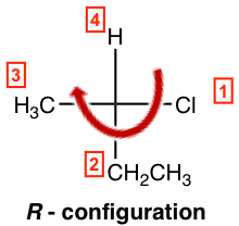
Entonces, el ejemplo aquí es un isómero R, y el nombre completo del compuesto es (R) -2-clorobutano.

Si el grupo de prioridad más baja está en un enlace horizontal (como ocurre en la siguiente estructura), determine la dirección de disminución de prioridad como en el paso 2, luego invierta la respuesta a manera opuesta, para obtener la configuración final.

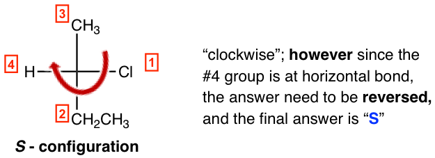
en sentido horario; sin embargo, dado que el grupo #4 es enlace horizontal, la respuesta necesita ser invertida, = S

Entonces, el ejemplo aquí es un isómero S, y el nombre completo del compuesto es (S) -2-clorobutano.

Ejercicios 5.6

Explique que ¿por qué en el paso 3 del procedimiento anterior, se debe revertir la respuesta para obtener la configuración final (real)?

Respuestas a las preguntas de práctica Capítulo 5

Ejercicios 5.7: Indicar la configuración de las siguientes estructuras.

Propiedades de la proyección Fisher:

1. Un interruptor (intercambio) de dos grupos en una proyección Fisher invierte la configuración, dos interruptores devuelven el isómero original.

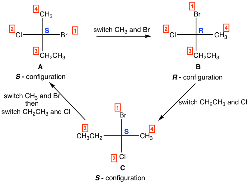
A=CH3 (arriba), Br (R), CH2CH3 (abajo), Cl (L), interruptor CH3 y Br (B) =R-configuración, interruptor CH2CH3, Cl (C) =S-configuración

Para las estructuras anteriores:

un interruptor de A conduce a B, A y B son enantiómeros;
un interruptor de B conduce a C, B y C son enantiómeros;
dos interruptores de cables C a A, A y C son idénticos.

2. Girar la proyección Fisher 180º obtener la misma estructura, con la configuración retenida.

Ambas son configuraciones S

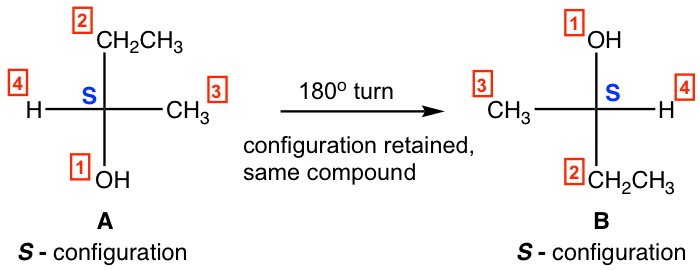
La rotación de 180º de A conduce a B, A y B son idénticos.

3. Girar la proyección Fisher 90º obtener la configuración invertida.

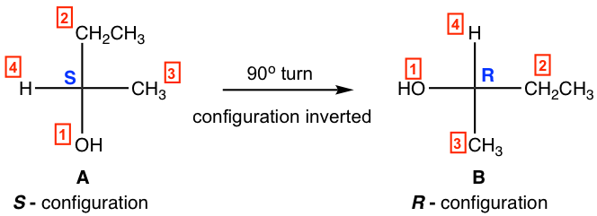
La configuración S se convierte en configuración R

La rotación de 90º de A conduce a B, A y B son enantiómeros.