2.4.4: Definición de funciones trigonométricas recíprocas inversas

Funciones de secante inversa, cosecante y cotangente.

Hasta ahora has tenido que lidiar con funciones trigonométricas, funciones recíprocas y funciones inversas. Ahora empezarás a ver funciones recíprocas inversas. Por ejemplo, ¿puedes calcular

\(\sec^{−1} \dfrac{2}{\sqrt{3}}\)

Resulta que esto se puede calcular fácilmente.

Funciones trigonométricas recíprocas inversas

Ya sabemos que la función cosecante es la recíproca de la función sinusoidal. Esto se utilizará para derivar el recíproco de la función sinusoidal inversa.

\(\begin{aligned} y&=\sin^{−1} x\\ x&=\sin y \\ \dfrac{1}{x}&=\csc y \\ \csc ^{−1} \dfrac{1}{x}&= y\\ \csc ^{−1} \dfrac{1}{x}&= \sin^{−1} x \end{aligned}\)

Porque cosecante y secante son inversos, también\(\sin^{−1}\dfrac{1}{x}=\csc ^{−1} x\) es cierto.

La identidad recíproca inversa para coseno y secante se puede probar usando el mismo proceso anterior. Sin embargo, recuerde que estas funciones inversas se definen mediante el uso de dominios restringidos y los recíprocos de estos inversos deben definirse con los intervalos de dominio y rango sobre los que son válidas las definiciones.

\(\sec^{−1}\dfrac{1}{x}=\cos ^{−1}x \leftrightarrow \cos ^{−1}\dfrac{1}{x}=\sec^{−1} x\)

Tangente y cotangente tienen una relación ligeramente diferente. Recordemos que la gráfica de cotangente difiere de la tangente por una reflexión sobre el eje y y un desplazamiento de\(\dfrac{\pi}{2}\). Como ecuación, esto se puede escribir como\(\cot x=−\tan\left(x−\dfrac{\pi}{2}\right)\). Tomando la inversa de esta función se mostrará la relación recíproca inversa entre arccotangente y arcotangente.

\ (\ begin {alineado}
y &=\ sin ^ {-1} x\
x &=\ sin y\
\ frac {1} {x} &=\ csc y\\
\ csc ^ {-1}\ frac {1} {x} &=y\
\ csc ^ {-1}\ frac {1} {x} &=\ sin ^ {-1} x
\ fin alineado}\)

Recuerda que tangente es una función impar, así que eso\(\tan(−x)=-\tan(x)\). Debido a que la tangente es impar, su inversa también es impar. Entonces, esto nos dice que\(\cot^{−1} x=\dfrac{\pi}{2}−\tan^{−1}x\) y\(\tan^{−1}x=\dfrac{\pi}{2}−\cot^{−1}x\). Para graficar arcsecant, arccosecant, y arccotangente en su calculadora utilizará estas identidades de conversión:\(\sec^{−1}x=\cos ^{−1} \dfrac{1}{x}\),\(\csc ^{−1} x=\sin^{−1}\dfrac{1}{x}\),\(\cot^{−1} x=\dfrac{\pi}{2}−\tan^{−1} x\). Nota: También es cierto que\(\cot^{−1}x=\tan^{−1}\dfrac{1}{x}\).

Encontrar la inversa

Encuentra la inversa de\(\sec^{−1}\sqrt{2}\)

Utilice la propiedad recíproca inversa. \(\sec^{−1}x=\cos ^{−1}\dfrac{1}{x}\rightarrow \sec^{−1} \sqrt{2}=\cos ^{−1}\dfrac{1}{\sqrt{2}}\)

Recordemos eso\(\dfrac{1}{\sqrt{2}}=\dfrac{1}{\sqrt{2}}\cdot \dfrac{\sqrt{2}}{\sqrt{2}}=\dfrac{\sqrt{2}}{2}\). Entonces,\(\sec^{−1}\sqrt{2}=\cos ^{−1}\dfrac{\sqrt{2}}{2}\), y eso lo sabemos\(\cos ^{−1}\dfrac{\sqrt{2}}{2}=\dfrac{\pi}{4}\). Por lo tanto,\(\sec^{−1}\sqrt{2}=\dfrac{\pi}{4}\).

Encontrar el valor exacto

Para cada uno de estos problemas, primero encuentra el recíproco y luego determina el ángulo a partir de ese (sin calculadora).

1. \(\sec^{−1}\sqrt{2}\)

\(\sec^{−1}\sqrt{2}=\cos ^{−1}\dfrac{\sqrt{2}}{2}\)Desde el círculo unitario, sabemos que la respuesta es\(\dfrac{\pi}{4}\).

2. \(\cot^{−1}(−\sqrt{3})\)

\(\cot^{−1}(−\sqrt{3})=\dfrac{\pi}{2}−\tan^{−1}(−\sqrt{3})\)Del círculo unitario, la respuesta es\(\dfrac{5\pi}{6}\).

3. \(\csc ^{−1}\dfrac{2\sqrt{3}}{3}\)

\(\csc ^{−1}\dfrac{2}{\sqrt{3}}3=\sin^{−1}\dfrac{\sqrt{3}}{2}\)Dentro de nuestro intervalo, hay una respuesta,\(\dfrac{\pi}{3}\).

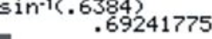
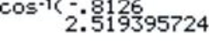
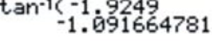
Uso de la tecnología

Asegúrate de que el MODO de tu calculadora sea RAD (radianes)

1. \(\arcsin 0.6384\)

Figura\(\PageIndex{1}\)

2. \(\arccos (−0.8126)\)

Figura\(\PageIndex{2}\)

3. \(\arctan (−1.9249)\)

Figura\(\PageIndex{3}\)

Ejemplo\(\PageIndex{1}\)

Anteriormente, se le pidió que evaluara\(\sec^{−1} \dfrac{2}{\sqrt{3}}\)

Solución

Puede comenzar con la propiedad recíproca inversa:

\(\sec^{−1}x=\cos ^{−1} \dfrac{1}{x}\)

Sustituir en valores por “x\)” da:

\(\sec^{−1}\dfrac{2}{\sqrt{3}}=\cos ^{−1}\dfrac{1}{\dfrac{2}{\sqrt{3}}}\)

Esto se puede reescribir como:

\(\cos ^{−1}\dfrac{\sqrt{3}}{2}\)

Y

\(\cos ^{−1} \dfrac{\sqrt{3}}{2}=\dfrac{\pi}{6}\)

Por lo tanto,

\(\sec^{−1} \dfrac{2}{\sqrt{3}}=\dfrac{\pi}{6}\)

Ejemplo\(\PageIndex{2}\)

Evaluar\(\sec^{−1}(−2)\)

Solución

\(\dfrac{2 \pi}{3}\)

Ejemplo\(\PageIndex{3}\)

Evaluar\(\cot^{−1}(−1)\)

Solución

\(−\dfrac{\pi}{4}\)

Ejemplo\(\PageIndex{4}\)

Evaluar\(\csc ^{−1}(\sqrt{2})\)

Solución

\(\dfrac{\pi}{4}\)

Revisar

Utilizando la tecnología, encuentra el valor en medida de radianes, de cada una de las siguientes.

1. \(\sin^{−1}(.345)\)
2. \(\cos ^{−1}(.87)\)
3. \(\csc ^{−1}(4)\)
4. \(\sec^{−1}(2.32)\)
5. \(\cot^{−1}(5.2)\)

Encuentra el valor exacto de cada expresión dentro del dominio restringido, sin calculadora.

6. \(\sec^{−1}(\dfrac{2\sqrt{3}}{3})\)
7. \(\csc ^{−1}(1)\)
8. \(\cot^{−1}(\sqrt{3})\)
9. \(\csc ^{−1}(2)\)
10. \(\sec^{−1}(\sqrt{2})\)
11. \(\cot^{−1}(1)\)
12. \(\cos ^{−1}\left(\dfrac{1}{2}\right)\)
13. \(\sec^{−1}(2)\)
14. \(\cot^{−1}\left(\dfrac{\sqrt{3}}{3}\right)\)
15. \(\sin^{−1}\left(\dfrac{\sqrt{3}}{2}\right)\)

Reseña (Respuestas)

Para ver las respuestas de Revisar, abra este archivo PDF y busque la sección 4.7.

El vocabulario

Término	Definición
función inversa	Las funciones inversas son funciones que se 'deshacen' entre sí. Formalmente\(f(x)\) y\(g(x)\) son funciones inversas si\(f(g(x))=g(f(x))=x\).
Función Recíproca	Una función recíproca es una función con la función padre\(y=\dfrac{1}{x}\).

Recursos adicionales

Video: Funciones recíprocas de trigonometría

Práctica: Definición de funciones trigonométricas recíprocas inversas