
14.2: Efectos de interacción
- Page ID
- 150224

\( \newcommand{\vecs}[1]{\overset { \scriptstyle \rightharpoonup} {\mathbf{#1}} } \)
\( \newcommand{\vecd}[1]{\overset{-\!-\!\rightharpoonup}{\vphantom{a}\smash {#1}}} \)
\( \newcommand{\id}{\mathrm{id}}\) \( \newcommand{\Span}{\mathrm{span}}\)
( \newcommand{\kernel}{\mathrm{null}\,}\) \( \newcommand{\range}{\mathrm{range}\,}\)
\( \newcommand{\RealPart}{\mathrm{Re}}\) \( \newcommand{\ImaginaryPart}{\mathrm{Im}}\)
\( \newcommand{\Argument}{\mathrm{Arg}}\) \( \newcommand{\norm}[1]{\| #1 \|}\)
\( \newcommand{\inner}[2]{\langle #1, #2 \rangle}\)
\( \newcommand{\Span}{\mathrm{span}}\)
\( \newcommand{\id}{\mathrm{id}}\)
\( \newcommand{\Span}{\mathrm{span}}\)
\( \newcommand{\kernel}{\mathrm{null}\,}\)
\( \newcommand{\range}{\mathrm{range}\,}\)
\( \newcommand{\RealPart}{\mathrm{Re}}\)
\( \newcommand{\ImaginaryPart}{\mathrm{Im}}\)
\( \newcommand{\Argument}{\mathrm{Arg}}\)
\( \newcommand{\norm}[1]{\| #1 \|}\)
\( \newcommand{\inner}[2]{\langle #1, #2 \rangle}\)
\( \newcommand{\Span}{\mathrm{span}}\) \( \newcommand{\AA}{\unicode[.8,0]{x212B}}\)
\( \newcommand{\vectorA}[1]{\vec{#1}} % arrow\)
\( \newcommand{\vectorAt}[1]{\vec{\text{#1}}} % arrow\)
\( \newcommand{\vectorB}[1]{\overset { \scriptstyle \rightharpoonup} {\mathbf{#1}} } \)
\( \newcommand{\vectorC}[1]{\textbf{#1}} \)
\( \newcommand{\vectorD}[1]{\overrightarrow{#1}} \)
\( \newcommand{\vectorDt}[1]{\overrightarrow{\text{#1}}} \)
\( \newcommand{\vectE}[1]{\overset{-\!-\!\rightharpoonup}{\vphantom{a}\smash{\mathbf {#1}}}} \)
\( \newcommand{\vecs}[1]{\overset { \scriptstyle \rightharpoonup} {\mathbf{#1}} } \)
\( \newcommand{\vecd}[1]{\overset{-\!-\!\rightharpoonup}{\vphantom{a}\smash {#1}}} \)
\(\newcommand{\avec}{\mathbf a}\) \(\newcommand{\bvec}{\mathbf b}\) \(\newcommand{\cvec}{\mathbf c}\) \(\newcommand{\dvec}{\mathbf d}\) \(\newcommand{\dtil}{\widetilde{\mathbf d}}\) \(\newcommand{\evec}{\mathbf e}\) \(\newcommand{\fvec}{\mathbf f}\) \(\newcommand{\nvec}{\mathbf n}\) \(\newcommand{\pvec}{\mathbf p}\) \(\newcommand{\qvec}{\mathbf q}\) \(\newcommand{\svec}{\mathbf s}\) \(\newcommand{\tvec}{\mathbf t}\) \(\newcommand{\uvec}{\mathbf u}\) \(\newcommand{\vvec}{\mathbf v}\) \(\newcommand{\wvec}{\mathbf w}\) \(\newcommand{\xvec}{\mathbf x}\) \(\newcommand{\yvec}{\mathbf y}\) \(\newcommand{\zvec}{\mathbf z}\) \(\newcommand{\rvec}{\mathbf r}\) \(\newcommand{\mvec}{\mathbf m}\) \(\newcommand{\zerovec}{\mathbf 0}\) \(\newcommand{\onevec}{\mathbf 1}\) \(\newcommand{\real}{\mathbb R}\) \(\newcommand{\twovec}[2]{\left[\begin{array}{r}#1 \\ #2 \end{array}\right]}\) \(\newcommand{\ctwovec}[2]{\left[\begin{array}{c}#1 \\ #2 \end{array}\right]}\) \(\newcommand{\threevec}[3]{\left[\begin{array}{r}#1 \\ #2 \\ #3 \end{array}\right]}\) \(\newcommand{\cthreevec}[3]{\left[\begin{array}{c}#1 \\ #2 \\ #3 \end{array}\right]}\) \(\newcommand{\fourvec}[4]{\left[\begin{array}{r}#1 \\ #2 \\ #3 \\ #4 \end{array}\right]}\) \(\newcommand{\cfourvec}[4]{\left[\begin{array}{c}#1 \\ #2 \\ #3 \\ #4 \end{array}\right]}\) \(\newcommand{\fivevec}[5]{\left[\begin{array}{r}#1 \\ #2 \\ #3 \\ #4 \\ #5 \\ \end{array}\right]}\) \(\newcommand{\cfivevec}[5]{\left[\begin{array}{c}#1 \\ #2 \\ #3 \\ #4 \\ #5 \\ \end{array}\right]}\) \(\newcommand{\mattwo}[4]{\left[\begin{array}{rr}#1 \amp #2 \\ #3 \amp #4 \\ \end{array}\right]}\) \(\newcommand{\laspan}[1]{\text{Span}\{#1\}}\) \(\newcommand{\bcal}{\cal B}\) \(\newcommand{\ccal}{\cal C}\) \(\newcommand{\scal}{\cal S}\) \(\newcommand{\wcal}{\cal W}\) \(\newcommand{\ecal}{\cal E}\) \(\newcommand{\coords}[2]{\left\{#1\right\}_{#2}}\) \(\newcommand{\gray}[1]{\color{gray}{#1}}\) \(\newcommand{\lgray}[1]{\color{lightgray}{#1}}\) \(\newcommand{\rank}{\operatorname{rank}}\) \(\newcommand{\row}{\text{Row}}\) \(\newcommand{\col}{\text{Col}}\) \(\renewcommand{\row}{\text{Row}}\) \(\newcommand{\nul}{\text{Nul}}\) \(\newcommand{\var}{\text{Var}}\) \(\newcommand{\corr}{\text{corr}}\) \(\newcommand{\len}[1]{\left|#1\right|}\) \(\newcommand{\bbar}{\overline{\bvec}}\) \(\newcommand{\bhat}{\widehat{\bvec}}\) \(\newcommand{\bperp}{\bvec^\perp}\) \(\newcommand{\xhat}{\widehat{\xvec}}\) \(\newcommand{\vhat}{\widehat{\vvec}}\) \(\newcommand{\uhat}{\widehat{\uvec}}\) \(\newcommand{\what}{\widehat{\wvec}}\) \(\newcommand{\Sighat}{\widehat{\Sigma}}\) \(\newcommand{\lt}{<}\) \(\newcommand{\gt}{>}\) \(\newcommand{\amp}{&}\) \(\definecolor{fillinmathshade}{gray}{0.9}\)Las variables ficticias también se pueden usar para estimar las formas en que el efecto de una variable difiere entre subconjuntos de casos. Este tipo de efectos generalmente se llaman interacciones”. Cuando se produce una interacción, el efecto de un XX depende del valor de otro. Típicamente, un modelo de OLS es aditivo, donde los BB se suman para predecir YY;
YI=a+bx1+bx2+bx3+bx4+eiyi=a+bx1+bx2+bx3+bx4+ei.
Sin embargo, un modelo de interacción tiene un efecto multiplicativo donde se multiplican dos de los IV;
YI=A+bx1+bx2+bx3*bx4+eiyi=a+bx1+bx2+bx3*bx4+ei.
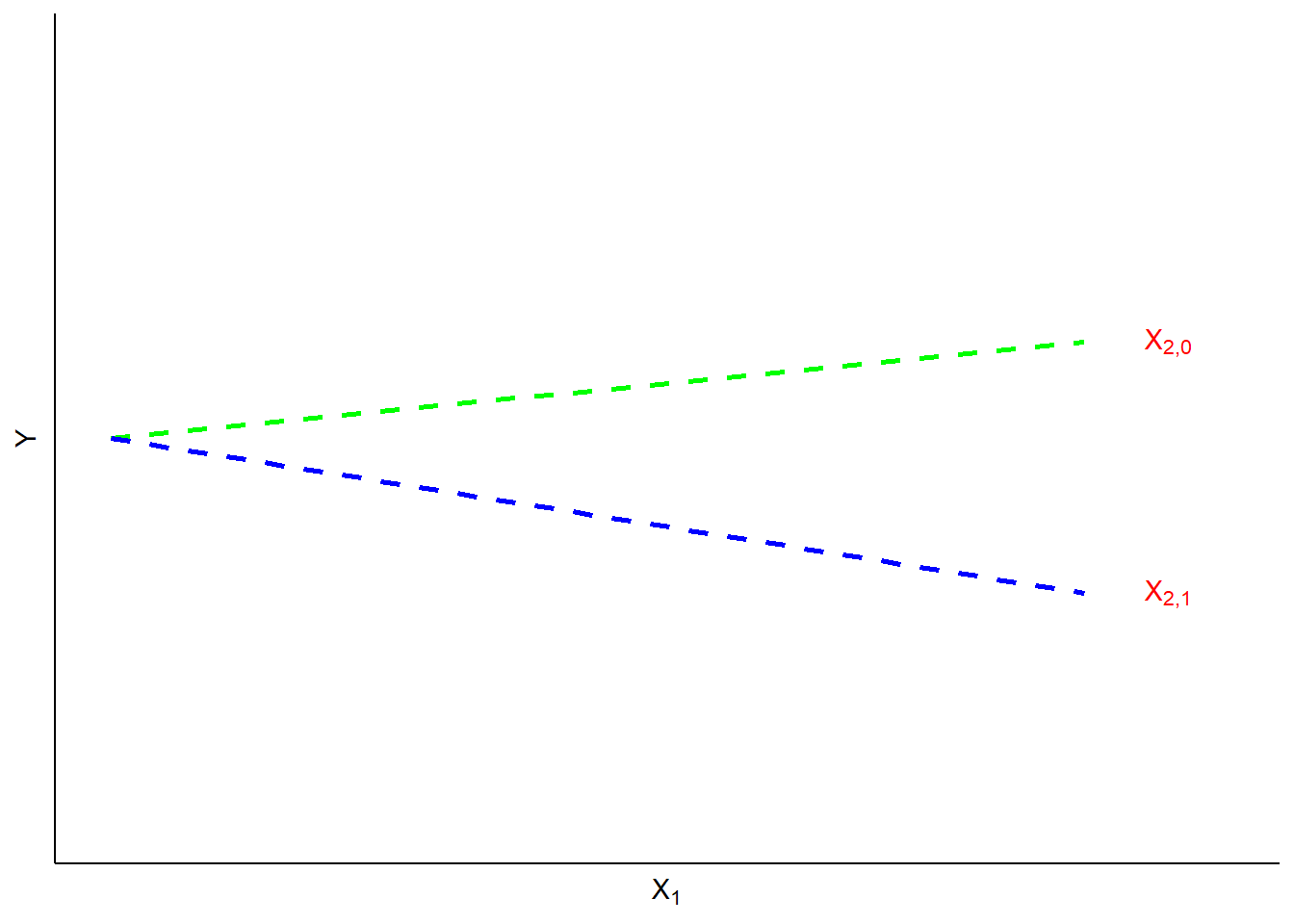
Un maniquí de pendiente” es un tipo especial de interacción en la que una variable ficticio interactúa con (multiplicada por) una variable de escala (ordinal o superior). Supongamos, por ejemplo, que planteaste la hipótesis de que los efectos de la política de ideología sobre los riesgos percibidos del cambio climático eran diferentes para hombres y mujeres. Quizás los hombres son más propensos que las mujeres a integrar consistentemente la ideología en las percepciones del riesgo del cambio En tal caso, una variable ficticio (0=mujeres, 1=hombres) podría ser interactuada con ideología (1=fuerte liberal, 7=fuerte conservadora) para predecir niveles de riesgo percibido de cambio climático (0=sin riesgo, 10=riesgo extremo). Si su interacción hipotética fuera correcta, observaría el tipo de patrón como se muestra en la Figura\(\PageIndex{2}\).
Podemos probar nuestra hipotética interacción en R, controlando los efectos de la edad y los ingresos.
ols2 <- lm(glbcc_risk ~ age + income + education + gender * ideol, data = ds.temp)
summary(ols2)
##
## Call:
## lm(formula = glbcc_risk ~ age + income + education + gender *
## ideol, data = ds.temp)
##
## Residuals:
## Min 1Q Median 3Q Max
## -8.718 -1.704 0.166 1.468 6.929
##
## Coefficients:
## Estimate Std. Error t value Pr(>|t|)
## (Intercept) 10.6004885194 0.3296900513 32.153 < 0.0000000000000002 ***
## age -0.0041366805 0.0036653120 -1.129 0.25919
## income -0.0000023222 0.0000009069 -2.561 0.01051 *
## education 0.0682885587 0.0299249903 2.282 0.02258 *
## gender 0.5971981026 0.2987398877 1.999 0.04572 *
## ideol -0.9591306050 0.0389448341 -24.628 < 0.0000000000000002 ***
## gender:ideol -0.1750006234 0.0597401590 -2.929 0.00343 **
## ---
## Signif. codes: 0 '***' 0.001 '**' 0.01 '*' 0.05 '.' 0.1 ' ' 1
##
## Residual standard error: 2.427 on 2264 degrees of freedom
## Multiple R-squared: 0.3664, Adjusted R-squared: 0.3647
## F-statistic: 218.2 on 6 and 2264 DF, p-value: < 0.00000000000000022Los resultados indican un efecto de interacción negativo y significativo para el género y la ideología. Consistente con nuestra hipótesis, esto significa que el efecto de la ideología sobre el riesgo de cambio climático es más pronunciado para los hombres que para las mujeres. Dicho de otra manera, la pendiente de la ideología es más pronunciada para los machos que para las hembras. Esto se muestra en la Figura\(\PageIndex{3}\).
ds.temp$gend.factor <- factor(ds.temp$gender, levels=c(0,1),labels=c("Female","Male"))
library(effects)
ols3 <- lm(glbcc_risk~ age + income + education + ideol * gend.factor, data = ds.temp)
plot(effect("ideol*gend.factor",ols3),ylim=0:10)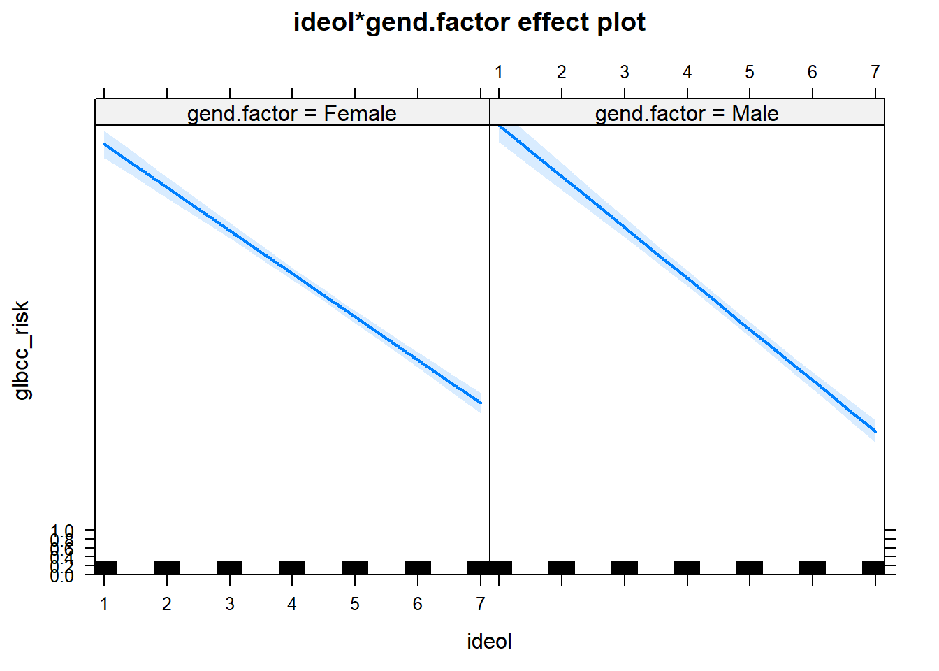
En resumen, las variables ficticias se suman en gran medida a la flexibilidad de la especificación del modelo OLS. Permiten la inclusión de variables categóricas y permiten probar hipótesis sobre interacciones de grupos con otros IV dentro del modelo. Este tipo de flexibilidad es una de las razones por las que los modelos de OLS son ampliamente utilizados por científicos sociales y analistas de políticas.