
5.8: Reglas de Kirchhoff
- Page ID
- 131713

\( \newcommand{\vecs}[1]{\overset { \scriptstyle \rightharpoonup} {\mathbf{#1}} } \)
\( \newcommand{\vecd}[1]{\overset{-\!-\!\rightharpoonup}{\vphantom{a}\smash {#1}}} \)
\( \newcommand{\id}{\mathrm{id}}\) \( \newcommand{\Span}{\mathrm{span}}\)
( \newcommand{\kernel}{\mathrm{null}\,}\) \( \newcommand{\range}{\mathrm{range}\,}\)
\( \newcommand{\RealPart}{\mathrm{Re}}\) \( \newcommand{\ImaginaryPart}{\mathrm{Im}}\)
\( \newcommand{\Argument}{\mathrm{Arg}}\) \( \newcommand{\norm}[1]{\| #1 \|}\)
\( \newcommand{\inner}[2]{\langle #1, #2 \rangle}\)
\( \newcommand{\Span}{\mathrm{span}}\)
\( \newcommand{\id}{\mathrm{id}}\)
\( \newcommand{\Span}{\mathrm{span}}\)
\( \newcommand{\kernel}{\mathrm{null}\,}\)
\( \newcommand{\range}{\mathrm{range}\,}\)
\( \newcommand{\RealPart}{\mathrm{Re}}\)
\( \newcommand{\ImaginaryPart}{\mathrm{Im}}\)
\( \newcommand{\Argument}{\mathrm{Arg}}\)
\( \newcommand{\norm}[1]{\| #1 \|}\)
\( \newcommand{\inner}[2]{\langle #1, #2 \rangle}\)
\( \newcommand{\Span}{\mathrm{span}}\) \( \newcommand{\AA}{\unicode[.8,0]{x212B}}\)
\( \newcommand{\vectorA}[1]{\vec{#1}} % arrow\)
\( \newcommand{\vectorAt}[1]{\vec{\text{#1}}} % arrow\)
\( \newcommand{\vectorB}[1]{\overset { \scriptstyle \rightharpoonup} {\mathbf{#1}} } \)
\( \newcommand{\vectorC}[1]{\textbf{#1}} \)
\( \newcommand{\vectorD}[1]{\overrightarrow{#1}} \)
\( \newcommand{\vectorDt}[1]{\overrightarrow{\text{#1}}} \)
\( \newcommand{\vectE}[1]{\overset{-\!-\!\rightharpoonup}{\vphantom{a}\smash{\mathbf {#1}}}} \)
\( \newcommand{\vecs}[1]{\overset { \scriptstyle \rightharpoonup} {\mathbf{#1}} } \)
\( \newcommand{\vecd}[1]{\overset{-\!-\!\rightharpoonup}{\vphantom{a}\smash {#1}}} \)
Incluso podemos adaptar las reglas de Kirchhoff para tratar con capacitores. Así, conecta un 24\(\text{V}\) battery across the circuit of Figure \(V.8\) – see Figure \(V.9\)
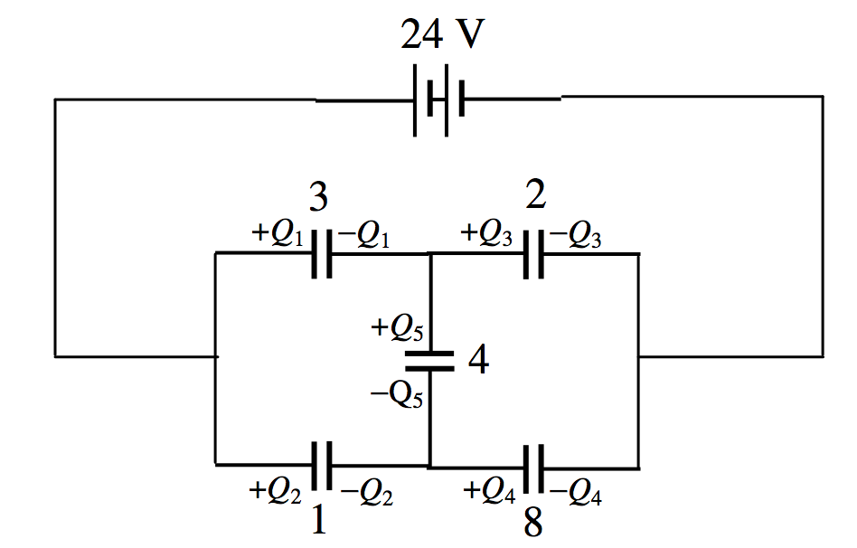
\(\text{FIGURE V.9}\)
Calcular la carga retenida en cada condensador. Podemos proceder de una manera muy similar a como lo hicimos en el Capítulo 4, aplicando la capacitancia equivalente de la segunda regla de Kirchhoff a tres circuitos cerrados, y luego conformando las cinco ecuaciones necesarias aplicando “la primera regla de Kirchhoff” a dos puntos. Así:
\[24-\frac{Q_2}{3}-\frac{Q_3}{2}=0,\label{5.8.1}\]
\[24-Q_2-\frac{Q_4}{8},\label{5.8.2}\]
\[\frac{Q_1}{3}-Q_2+\frac{Q_5}{4}=0,\]
\[Q_1=Q_3+Q_5,\]
\[Q_4=Q_2+Q_5,\]
Hago las soluciones
\[Q_1=+41.35\mu \text{C},\,Q_2=+19.01\mu \text{C},\,Q_3=+20.44\mu \text{C},\,Q_4 = +39.92 \mu \text{C},\,Q_5 =20.91 \mu \text{C}.\]