
13.1: Corriente alterna en una inductancia
- Page ID
- 131872

\( \newcommand{\vecs}[1]{\overset { \scriptstyle \rightharpoonup} {\mathbf{#1}} } \)
\( \newcommand{\vecd}[1]{\overset{-\!-\!\rightharpoonup}{\vphantom{a}\smash {#1}}} \)
\( \newcommand{\id}{\mathrm{id}}\) \( \newcommand{\Span}{\mathrm{span}}\)
( \newcommand{\kernel}{\mathrm{null}\,}\) \( \newcommand{\range}{\mathrm{range}\,}\)
\( \newcommand{\RealPart}{\mathrm{Re}}\) \( \newcommand{\ImaginaryPart}{\mathrm{Im}}\)
\( \newcommand{\Argument}{\mathrm{Arg}}\) \( \newcommand{\norm}[1]{\| #1 \|}\)
\( \newcommand{\inner}[2]{\langle #1, #2 \rangle}\)
\( \newcommand{\Span}{\mathrm{span}}\)
\( \newcommand{\id}{\mathrm{id}}\)
\( \newcommand{\Span}{\mathrm{span}}\)
\( \newcommand{\kernel}{\mathrm{null}\,}\)
\( \newcommand{\range}{\mathrm{range}\,}\)
\( \newcommand{\RealPart}{\mathrm{Re}}\)
\( \newcommand{\ImaginaryPart}{\mathrm{Im}}\)
\( \newcommand{\Argument}{\mathrm{Arg}}\)
\( \newcommand{\norm}[1]{\| #1 \|}\)
\( \newcommand{\inner}[2]{\langle #1, #2 \rangle}\)
\( \newcommand{\Span}{\mathrm{span}}\) \( \newcommand{\AA}{\unicode[.8,0]{x212B}}\)
\( \newcommand{\vectorA}[1]{\vec{#1}} % arrow\)
\( \newcommand{\vectorAt}[1]{\vec{\text{#1}}} % arrow\)
\( \newcommand{\vectorB}[1]{\overset { \scriptstyle \rightharpoonup} {\mathbf{#1}} } \)
\( \newcommand{\vectorC}[1]{\textbf{#1}} \)
\( \newcommand{\vectorD}[1]{\overrightarrow{#1}} \)
\( \newcommand{\vectorDt}[1]{\overrightarrow{\text{#1}}} \)
\( \newcommand{\vectE}[1]{\overset{-\!-\!\rightharpoonup}{\vphantom{a}\smash{\mathbf {#1}}}} \)
\( \newcommand{\vecs}[1]{\overset { \scriptstyle \rightharpoonup} {\mathbf{#1}} } \)
\( \newcommand{\vecd}[1]{\overset{-\!-\!\rightharpoonup}{\vphantom{a}\smash {#1}}} \)
En la Figura vemos una corriente aumentando hacia la derecha y pasando por un inductor. Como consecuencia de la inductancia, se indujo una contraCEM, con los signos como se indica. Denoto la parte posterior EMF por\(V = V_A - V_B\). El EMF posterior es dado por\(V=L\dot I\).
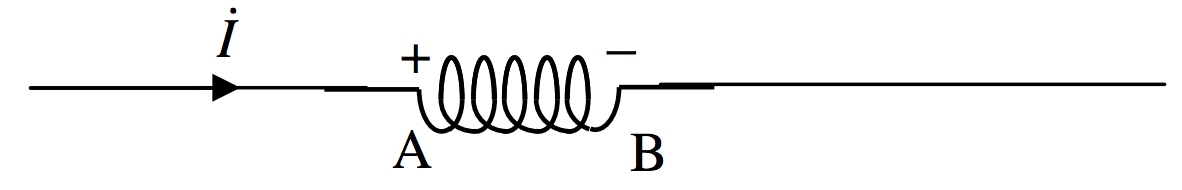
FIGURA\(\text{XIII.1}\)
Ahora supongamos que la corriente es una corriente alterna dada por
\[\label{13.1.1}I=\hat{I}\sin \omega t.\]
En ese caso\(\dot I = \hat{I}\omega \cos \omega t\), and therefore the back EMF is
\[\label{13.1.2}V=\hat{I}L\omega \cos \omega t,\]
que se puede escribir
\[\label{13.1.3}V=\hat{V}\cos \omega t,\]
donde el voltaje pico es
\[\label{13.1.4}\hat{V}=L\omega \hat{I}\]
y, por supuesto\(V_{\text{RMS}}=L\omega I_{\text{RMS}}\) (Section 13.11).
La cantidad\(L\omega\) se llama reactancia inductiva\(X_L\) . Se expresa en ohmios (verifique las dimensiones), y, cuanto mayor sea la frecuencia, mayor será la reactancia. (La frecuencia\(\nu\) es\(\omega/(2\pi)\). )
La comparación de las ecuaciones\ ref {13.1.1} y\ ref {13.1.3} muestra que la corriente y el voltaje están desfasados, y que\(V\) leads on \(I\) by 90o, as shown in Figure XIII.2.
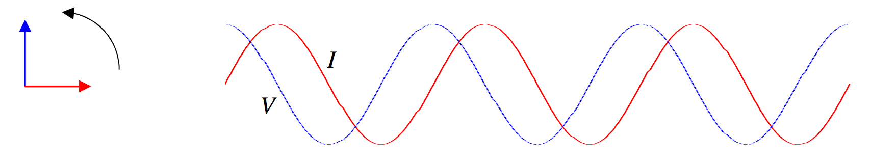
FIGURA\(\text{XIII.2}\)