
14.12: Otro Ejemplo
- Page ID
- 131948

\( \newcommand{\vecs}[1]{\overset { \scriptstyle \rightharpoonup} {\mathbf{#1}} } \)
\( \newcommand{\vecd}[1]{\overset{-\!-\!\rightharpoonup}{\vphantom{a}\smash {#1}}} \)
\( \newcommand{\id}{\mathrm{id}}\) \( \newcommand{\Span}{\mathrm{span}}\)
( \newcommand{\kernel}{\mathrm{null}\,}\) \( \newcommand{\range}{\mathrm{range}\,}\)
\( \newcommand{\RealPart}{\mathrm{Re}}\) \( \newcommand{\ImaginaryPart}{\mathrm{Im}}\)
\( \newcommand{\Argument}{\mathrm{Arg}}\) \( \newcommand{\norm}[1]{\| #1 \|}\)
\( \newcommand{\inner}[2]{\langle #1, #2 \rangle}\)
\( \newcommand{\Span}{\mathrm{span}}\)
\( \newcommand{\id}{\mathrm{id}}\)
\( \newcommand{\Span}{\mathrm{span}}\)
\( \newcommand{\kernel}{\mathrm{null}\,}\)
\( \newcommand{\range}{\mathrm{range}\,}\)
\( \newcommand{\RealPart}{\mathrm{Re}}\)
\( \newcommand{\ImaginaryPart}{\mathrm{Im}}\)
\( \newcommand{\Argument}{\mathrm{Arg}}\)
\( \newcommand{\norm}[1]{\| #1 \|}\)
\( \newcommand{\inner}[2]{\langle #1, #2 \rangle}\)
\( \newcommand{\Span}{\mathrm{span}}\) \( \newcommand{\AA}{\unicode[.8,0]{x212B}}\)
\( \newcommand{\vectorA}[1]{\vec{#1}} % arrow\)
\( \newcommand{\vectorAt}[1]{\vec{\text{#1}}} % arrow\)
\( \newcommand{\vectorB}[1]{\overset { \scriptstyle \rightharpoonup} {\mathbf{#1}} } \)
\( \newcommand{\vectorC}[1]{\textbf{#1}} \)
\( \newcommand{\vectorD}[1]{\overrightarrow{#1}} \)
\( \newcommand{\vectorDt}[1]{\overrightarrow{\text{#1}}} \)
\( \newcommand{\vectE}[1]{\overset{-\!-\!\rightharpoonup}{\vphantom{a}\smash{\mathbf {#1}}}} \)
\( \newcommand{\vecs}[1]{\overset { \scriptstyle \rightharpoonup} {\mathbf{#1}} } \)
\( \newcommand{\vecd}[1]{\overset{-\!-\!\rightharpoonup}{\vphantom{a}\smash {#1}}} \)
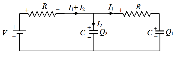
\(\text{FIGURE XIV.1}\)
El circuito en la Figura\(\text{XIV.1}\) contains two equal resistances, two equal capacitances, and a battery. The battery is connected at time \(t=0\). Find the charges held by the capacitors after time \(t\).
Aplica la segunda regla de Kirchhoff a cada mitad:
\[(\dot Q_1 + \dot Q_2)RC + Q_2 = CV, \tag{14.12.1}\]
y\[\dot Q_1 RC + Q_1 - Q_2 = 0.\tag{14.12.2}\]
Eliminar\(Q_2\):
\[R^2C^2\ddot Q_1 + 3 RC Q_1 + Q_1 = CV. \tag{14.12.3}\]
Transformar, con\(Q_1\) and \(\dot Q_1\) initially zero:
\[(R^2C^2s^2 + 3RCs + 1) \bar{Q_1} = \frac{CV}{s}.\tag{14.12.4}\]
Es decir,\[R^2C\bar{Q_1} = \frac{1}{s(s^2 + 3as + a^2)} \cdot V , \tag{14.12.5}\]
donde\[a=1/(RC). \tag{14.12.6}\]
Eso es\[R^2C \bar{Q_1}= \frac{1}{s(s+2.618a)(s+0.382a)}V. \tag{14.12.7}\]
Fracciones parciales:\[R^2C\bar{Q_1} = \left[\frac{1}{s} + \frac{0.1708}{s+2.618a} - \frac{1.1708}{s+0.382a} \right] \frac{V}{a^2}. \tag{14.12.8}\]
Es decir,\[\bar{Q_1} = \left[ \frac{1}{s} + \frac{0.1708}{s+2.618a} - \frac{1.1708}{s+0.382a} \right]CV. \tag{14.12.9}\]
Transformación inversa:\[Q_1 = \left[ 1 + 0.1708e^{-2.618t/(RC)} - 1.1708e^{-0.382t/(RC)} \right]. \tag{14.12.10}\]
La corriente se puede encontrar por diferenciación.
Dejo al lector eliminar\(Q_1\) from equations 14.12.1 and 2 and hence to show that
\[Q_2 = \left[1 - 0.2764 e^{-2.618 t/(RC)} - 0.7236 e^{-0.382 t/(RC)} \right]. \tag{14.12.11}\]