22A: Centro de Masa, Momento de Inercia

Un error que surge en el cálculo de los momentos de inercia, involucra el Teorema del Eje Paralelo. El error es intercambiar el momento de inercia del eje a través del centro de masa, con el paralelo a ese, al aplicar el Teorema del Eje Paralelo. Reconocer que el subíndice “CM” en el teorema del eje paralelo significa “centro de masa” ayudará a evitar este error. También, una comprobación de la respuesta, para asegurarse de que el valor del momento de inercia con respecto al eje a través del centro de masa es menor que el otro momento de inercia, atrapará el error.

Centro de Masa

Considera dos partículas, que tienen una y la misma masa m, cada una de las cuales se encuentra en una posición diferente en el eje x de un sistema de coordenadas cartesianas.

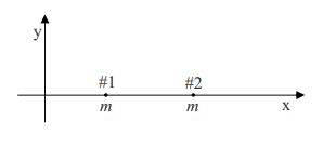
El sentido común te dice que la posición promedio del material que compone las dos partículas está a medio camino entre las dos partículas. El sentido común es correcto. Damos el nombre de “centro de masa” a la posición promedio del material que constituye una distribución, y el centro de masa de un par de partículas de la misma masa está de hecho a medio camino entre las dos partículas.

¿Qué tal si una de las partículas es más masiva que la otra? Uno esperaría que el centro de masa estuviera más cerca de la partícula más masiva, y nuevamente, uno tendría razón. Para determinar la posición del centro de masa de la distribución de la materia en tal caso, calculamos una suma ponderada de las posiciones de las partículas en la distribución, donde el factor de ponderación para una partícula dada es esa fracción, de la masa total, que es la masa propia de la partícula. Así, para dos partículas en el\(x\) eje, una de masa\(m_1\), en\(x_1\), y la otra de masa\(m_2\), en\(x_2\),

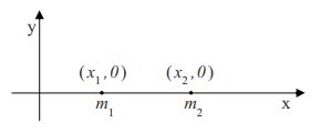
la posición\(\bar{x}\) del centro de masa viene dada por

\[\bar{x}=\frac{m_1}{m_1+m_2} x_1+ \frac{m_2}{m_1+m_2} x_2 \label{22-1}\]

Obsérvese que cada factor de ponderación es una fracción propia y que la suma de los factores de ponderación es siempre 1. También tenga en cuenta que si, por ejemplo,\(m_1\) es mayor que\(m_2\), entonces la posición\(x_1\) de la partícula 1 contará más en la suma, asegurando así que el centro de masa se encuentre más cerca de la partícula más masiva (como sabemos que debe ser). Obsérvese además que si\(m_1=m_2\), cada factor de ponderación es\(\frac{1}{2}\), como es evidente cuando sustituimos m por ambos\(m_1\) y\(m_2\) en la Ecuación\(\ref{22-1}\):

\[\bar{x}=\dfrac{m}{m+m} x_1+ \frac{m}{m+m} x_2 \]

\[\bar{x}=\dfrac{1}{2}x_1+\frac{1}{2}x_2 \]

\[\bar{x}=\dfrac{x_1+x_2}{2} \]

Se encuentra que el centro de masa está a medio camino entre las dos partículas, justo donde el sentido común nos dice que tiene que estar.

El centro de masa de una varilla delgada

Muy a menudo, cuando se requiere el hallazgo de la posición del centro de masa de una distribución de partículas, la distribución de partículas es el conjunto de partículas que conforman un cuerpo rígido. El cuerpo rígido más fácil para el que calcular el centro de masa es la varilla delgada porque se extiende en una sola dimensión. (Aquí, discutimos una varilla delgada ideal. Una varilla delgada física debe tener un diámetro distinto de cero. La varilla delgada ideal, sin embargo, es una buena aproximación a la varilla delgada física siempre que el diámetro de la varilla sea pequeño en comparación con su longitud).

En el caso más simple, el cálculo de la posición del centro de masa es trivial. El caso más simple involucra una varilla delgada uniforme. Una varilla delgada uniforme es aquella para la cual la densidad de masa lineal\(\mu\), la masa por longitud de la varilla, tiene uno y el mismo valor en todos los puntos de la varilla. El centro de masa de una varilla uniforme está en el centro de la varilla. Entonces, por ejemplo, el centro de masa de una varilla uniforme que se extiende a lo largo del eje x de\(x=0\) a\(x=L\) está en (L/2, 0).

La densidad de masa lineal\(\mu\), típicamente llamada densidad lineal cuando el contexto es claro, es una medida de lo estrechamente empaquetadas que están las partículas elementales que componen la varilla. Donde la densidad lineal es alta, las partículas están muy juntas.

Para imaginar lo que se entiende por una varilla no uniforme, una varilla cuya densidad lineal es función de la posición, imagine una varilla delgada hecha de una aleación que consiste en plomo y aluminio. Además imagine que el porcentaje de plomo en la varilla varía suavemente de 0% en un extremo de la varilla a 100% en el otro. La densidad lineal de dicha varilla sería una función de la posición a lo largo de la longitud de la varilla. Un segmento de un milímetro de la varilla en una posición tendría una masa diferente a la de un segmento de un milímetro de la varilla en una posición diferente.

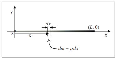
A las personas con cierta exposición al cálculo les resulta más fácil entender qué es la densidad lineal que los individuos privados de cálculo porque la densidad lineal es solo la relación entre la cantidad de masa en un segmento de varilla y la longitud del segmento, en el límite ya que la longitud del segmento va a cero. Considera una varilla que se extiende de\(0\) a\(L\) lo largo del\(x\) eje. Ahora supongamos que\(m_s(x)\) es la masa de ese segmento de la varilla que se extiende desde\(0\)\(x\) donde\(x\ge0\) pero\(x<L\). Entonces, la densidad lineal de la varilla en cualquier punto x a lo largo de la varilla, solo se\(\frac{dm_s}{dx}\) evalúa al valor de\(x\) en cuestión.

Ahora que se tiene una buena idea de lo que queremos decir con densidad de masa lineal, vamos a ilustrar cómo se determina la posición del centro de masa de una varilla delgada no uniforme por medio de un ejemplo.

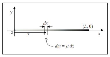
Encuentra la posición del centro de masa de una varilla delgada que se extiende desde\(0\) to \(.890\)m along the \(x\) axis of a Cartesian coordinate system and has a linear density given by \(\mu(x)=0.650\frac{kg}{m^3}x^2\).

Solution

In order to be able to determine the position of the center of mass of a rod with a given length and a given linear density as a function of position, you first need to be able to find the mass of such a rod. To do that, one might be tempted to use a method that works only for the special case of a uniform rod, namely, to try using \(m=\mu L\) with \(L\) being the length of the rod. The problem with this is, that \(\mu\) varies along the entire length of the rod. What value would one use for \(\mu\)? One might be tempted to evaluate the given \(\mu\) at \(x=L\) and use that, but that would be acting as if the linear density were constant at \(\mu=\mu (L)\). It is not. In fact, in the case at hand, \(\mu(L)\) is the maximum linear density of the rod, it only has that value at one point on the rod.

What we can do is to say that the infinitesimal amount of mass \(dm\) in a segment \(dx\) of the rod is \(\mu dx\). Here we are saying that at some position \(x\) on the rod, the amount of mass in the infinitesimal length \(dx\) of the rod is the value of \(\mu\) at that \(x\) value, times the infinitesimal length \(dx\). Here we don’t have to worry about the fact that \(\mu\) changes with position since the segment \(dx\) is infinitesimally long, meaning, essentially, that it has zero length, so the whole segment is essentially at one position \(x\) and hence the value of \(\mu\) at that \(x\) is good for the whole segment \(dx\).

\[dm=\mu (x) dx \label{22-2} \]

Now this is true for any value of \(x\), but it just covers an infinitesimal segment of the rod at \(x\). To get the mass of the whole rod, we need to add up all such contributions to the mass. Of course, since each \(dm\) corresponds to an infinitesimal length of the rod, we will have an infinite number of terms in the sum of all the \(dm\)’s. An infinite sum of infinitesimal terms, is an integral.

\[\int dm=\int_{0}{L} \mu (x) dx \label{22-3}\]

where the values of \(x\) have to run from \(0\) to \(L\) to cover the length of the rod, hence the limits on the right. Now the mathematicians have provided us with a rich set of algorithms for evaluating integrals, and indeed we will have to reach into that toolbox to evaluate the integral on the right, but to evaluate the integral on the left, we cannot, should not, and will not turn to such an algorithm. Instead, we use common sense and our conceptual understanding of what the integral on the left means. In the context of the problem at hand, \(\int dm\) means “the sum of all the infinitesimal bits of mass making up the rod.” Now, if you add up all the infinitesimal bits of mass making up the rod, you get the mass of the rod. So \(\int dm\) is just the mass of the rod, which we will call \(m\). Equation \(\ref{22-3}\) then becomes

\[m=\int_{0}{L} \mu(x) dx \label{22-4}\]

Replacing \(\mu (x)\) with the given expression for the linear density \(\mu=0.650 \frac{kg}{m^3} x^2\) which I choose to write as \(\mu=bx^2\) with \(b\) being defined by \(b=0.650 \frac{kg}{m^3}\) we obtain

\[m=\int_{0}{L}bx^2dx\]

Factoring out the constant yields

\[m=b\int_{0}{L}x^2dx\]

When integrating the variable of integration raised to a power all we have to do is increase the power by one and divide by the new power. This gives

\[m=b\frac{x^3}{3} \Big |_0^L \]

Evaluating this at the lower and upper limits yields

\[ m=b(\frac{L^3}{3}-\frac{0^3}{3}) \]

\[m=\frac{bL^3}{3} \]

The value of \(L\) is given as \(0.890 m\) and we defined \(b\) to be the constant \(0.650 \frac{kg}{m^3}\) in the given expression for \(\mu\), \(\mu=0.650\frac{kg}{m^3} x^2\), so

\[ m=\frac{0.650 \frac{kg}{m^3} (0.890m)^3}{3} \]

\[m=0.1527kg\]

That’s a value that will come in handy when we calculate the position of the center of mass. Now, when we calculated the center of mass of a set of discrete particles (where a discrete particle is one that is by itself, as opposed, for instance, to being part of a rigid body) we just carried out a weighted sum in which each term was the position of a particle times its weighting factor and the weighting factor was that fraction, of the total mass, represented by the mass of the particle. We carry out a similar procedure for a continuous distribution of mass such as that which makes up the rod in question. Let’s start by writing one single term of the sum. We’ll consider an infinitesimal length \(dx\) of the rod at a position \(x\) along the length of the rod. The position, as just stated, is \(x\), and the weighting factor is that fraction of the total mass \(m\) of the rod that the mass \(dm\) of the infinitesimal length \(dx\) represents. That means the weighting factor is \(\frac{dm}{m}\), so, a term in our weighted sum of positions looks like:

\[\frac{dm}{m} x\]

Now, \(dm\) can be expressed as \(\mu\)\(dx\) so our expression for the term in the weighted sum can be written as

\[ \frac{\mu dx}{m} x\]

That’s one term in the weighted sum of positions, the sum that yields the position of the center of mass. The thing is, because the value of \(x\) is unspecified, that one term is good for any infinitesimal segment of the bar. Every term in the sum looks just like that one. So we have an expression for every term in the sum. Of course, because the expression is for an infinitesimal length \(dx\) of the rod, there will be an infinite number of terms in the sum. So, again we have an infinite sum of infinitesimal terms. That is, again we have an integral. Our expression for the position of the center of mass is:

\[\bar{x}=\int_{0}{L} \frac{\mu dx}{m} x\]

Substituting the given expression \(\mu (x)=0.650\frac{kg}{m^3} x^2\) for \(\mu\), which we again write as \(\mu=bx^2\) with \(b\) being defined by \(b=0.650\frac{kg}{m^3} \), yields

\[\bar{x}=\int_{0}{L} \frac{bx^2 dx}{m} x\]

Rearranging and factoring the constants out gives

\[\bar{x}=\frac{b}{m} \int_{0}{L} x^3 dx\]

Next we carry out the integration

\[\bar{x}=\frac{b}{m} \frac{x^4}{4} \Big |_0^L\]

\[\bar{x}=\frac{b}{m} (\frac{L^4}{4}-\frac{0^4}{4})\]

\[\bar{x}=\frac{bL^4}{4m} \]

Now we substitute values with units; the mass m of the rod that we found earlier, the constant \(b\) that we defined to simplify the appearance of the linear density function, and the given length \(L\) of the rod:

\[\bar{x}=\frac{(0.650\frac{kg}{m^3})(0.890m)^4}{4(0.1527kg)}\]

\[ \bar{x}=0.668m\]

This is our final answer for the position of the center of mass. Note that it is closer to the denser end of the rod, as we would expect. The reader may also be interested to note that had we substituted the expression \(m=\frac{bL^3}{3}\) that we derived for the mass, rather than the value we obtained when we evaluated that expression, our expression for \(\bar{x}\) would have simplified to \(\frac{3}{4} L\) which evaluates to \(\bar{x}=0.668m\), the same result as the one above.

Momento de inercia, también conocido como inercia rotacional

Ya se sabe que el momento de inercia de un objeto rígido, con respecto a un eje de rotación especificado, depende de la masa de ese objeto, y de cómo se distribuye esa masa en relación con el eje de rotación. De hecho, sabes que si la masa se empaqueta cerca del eje de rotación, el objeto tendrá un momento de inercia menor que si la misma masa estuviera más extendida en relación con el eje de rotación. Cuantifiquemos estas ideas. (Cuantificar, en este contexto, significa poner en forma de ecuación.)

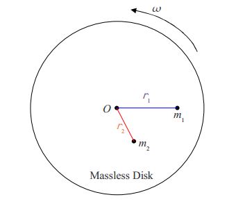
Comenzamos construyendo, en nuestra mente, un objeto idealizado para el cual la masa se concentra en una sola ubicación que no está en el eje de rotación: Imagínese un disco sin masa que gira con velocidad angular w alrededor de un eje a través del centro del disco y perpendicular a sus caras. Que haya una partícula de masa m incrustada en el disco a una\(r\) distancia del eje de rotación. Así es como se ve desde un punto de vista sobre el eje de rotación, a cierta distancia del disco:

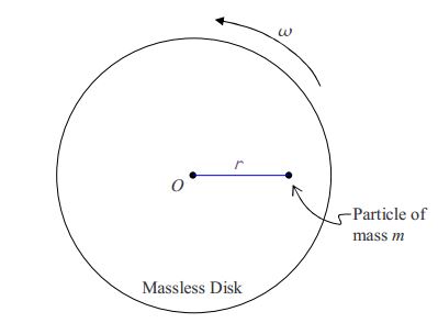
donde el eje de rotación está marcado con un\(O\). Debido a que el disco es sin masa, llamamos al momento de inercia de la construcción, el momento de inercia de una partícula, con respecto a la rotación alrededor de un eje desde el que la partícula está a una distancia\(r\).

Sabiendo que la velocidad de la partícula se puede expresar ya\(v=r\omega\) que puede mostrarse cómo\(I\) debe definirse para que la expresión de energía cinética\(K=\frac{1}{2} I \omega^2\) para el objeto, visto como un cuerpo rígido giratorio, sea la misma que la expresión de energía cinética\(K=\frac{1}{2} m v^2\) para la partícula moviéndose a través del espacio en un círculo. Cualquiera de los dos puntos de vista es válido por lo que ambos puntos de vista deben producir la misma energía cinética. Por favor, siga adelante y derive lo que\(I\) debe ser y luego regrese y lea la derivación a continuación.

Aquí está la derivación:

Dado eso\(K=\frac{1}{2} m v^2\), reemplazamos\(v\) por\(r\omega\).

Esto da\(K=\frac{1}{2} m (r\omega)^2\)

que se puede escribir como

\[K=\frac{1}{2} (mr^2) \omega^2\]

Para que esto sea equivalente a

\[ K=\frac{1}{2} I \omega^2\]

debemos tener

\[ I=mr^2 \label{22-5}\]

Este es nuestro resultado para el momento de inercia de una partícula de masa\(m\), con respecto a un eje de rotación desde el que la partícula está a una distancia\(r\).

Ahora supongamos que tenemos dos partículas incrustadas en nuestro disco sin masa, una de masa\(m_1\) a una\(r_1\) distancia del eje de rotación y otra de masa\(m_2\) a una\(r_2\) distancia del eje de rotación.

El momento de inercia del primero por sí mismo sería

\[I_1=m_1 r_1^2\]

y el momento de inercia de la segunda partícula por sí mismo sería

\[I_2=m_2 r_2^2\]

El momento total de inercia de las dos partículas incrustadas en el disco sin masa es simplemente la suma de los dos momentos individuales de inercia.

\[I=I_1+I_2\]

\[I=m_1 r_1^2+m_2 r_2^2\]

Este concepto puede extenderse para incluir cualquier número de partículas. Para cada partícula adicional, uno simplemente incluye otro\(m_i r_i^2\) término en la suma donde\(m_i\) está la masa de la partícula adicional y\(r_i\) es la distancia que la partícula adicional está del eje de rotación. En el caso de un objeto rígido, subdividimos el objeto en un conjunto infinito de elementos de masa infinitesimales\(dm\). Cada elemento de masa aporta una cantidad de momento de inercia

\[dI=r^2dm \label{22-6}\]

al momento de inercia del objeto, donde\(r\) está la distancia que el elemento de masa particular se encuentra desde el eje de rotación.

Encuentra el momento de inercia de la varilla en Ejemplo\(\ref{22-1}\) with respect to rotation about the z axis.

Solution

In Example \(\ref{22-1}\), the linear density of the rod was given as \(\mu=0.650 \frac{kg}{m^3}x^2\). To reduce the number of times we have to write the value in that expression, we will write it as \(\mu=bx^2\) with \(b\) being defined as \(b=0.650 \frac{kg}{m^3}\).

The total moment of inertia of the rod is the infinite sum of the infinitesimal contributions

\[dI=r^2 dm \label{22-6} \]

from each and every mass element dm making up the rod.

In the diagram, we have indicated an infinitesimal element \(dx\) of the rod at an arbitrary position on the rod. The z axis, the axis of rotation, looks like a dot in the diagram and the distance \(r\) in \(dI=r^2 dm\), the distance that the bit of mass under consideration is from the axis of rotation, is simply the abscissa x of the position of the mass element. Hence, equation \(\ref{22-6}\) for the case at hand can be written as

\[dI=x^2 dm\]

which we copy here

\[dI=x^2 dm\]

By definition of the linear mass density \(\mu\), the infinitesimal mass \(dm\) can be expressed as \(dm = \mu dx\). Substituting this into our expression for \(dI\) yields

\[dI=x^2 \mu dx\]

Now \(\mu\) was given as \(bx^2\) (with \(b\) actually being the symbol that I chose to use to represent the given constant \(0.650 \frac{kg}{m^3}\)). Substituting \(bx^2\) in for \(\mu\) in our expression for \(dI\) yields

\[dI=x^2(bx^2)dx\]

\[dI=bx^4dx\]

This expression for the contribution of an element \(dx\) of the rod to the total moment of inertia of the rod is good for every element \(dx\) of the rod. The infinite sum of all such infinitesimal contributions is thus the integral

\[\int dI=\int_{0}{L} bx^4 dx\]

Again, as with our last integration, on the left, we have not bothered with limits of integration— the infinite sum of all the infinitesimal contributions to the moment of inertia is simply the total moment of inertia.

\[I=\int_{0}{L}bx^4 dx\]

On the right we use the limits of integration \(0\) to \(L\) to include every element of the rod which extends from \(x=0\) to \(x=L\), with L given as \(0.890 m\). Factoring out the constant \(b\) gives us

\[I=b \int_{0}{L}x^4 dx\]

Now we carry out the integration:

\[I=b\frac{x^5}{5} \Big|_0^L\]

\[I=b(\frac{L^5}{5}-\frac{0^5}{5})\]

\[I=b\frac{L^5}{5}\]

Substituting the given values of \(b\) and \(L\) yields:

\[I=0.650 \frac{kg}{m^3} \frac{(0.890m)^5}{5}\]

\[I=0.0726 kg\cdot m^2\]

Teorema del Eje Paralelo

Nosotros declaramos, sin pruebas, el teorema del eje paralelo:

\[I=I_{cm}+md^2 \label{22-7}\]

en el que:

• \(I\)es el momento de inercia de un objeto con respecto a un eje desde el cual el centro de masa del objeto está a una distancia\(d\).
• \(I_{cm}\)es el momento de inercia del objeto con respecto a un eje que es paralelo al primer eje y pasa por el centro de masa.
• \(m\)es la masa del objeto
• \(d\)es la distancia entre los dos ejes.

El teorema del eje paralelo relaciona el momento\(I_{CM}\) de inercia de un objeto, con respecto a un eje a través del centro de masa del objeto, con el momento de inercia I del mismo objeto, con respecto a un eje que es paralelo al eje a través del centro de masa y se encuentra a una distancia d del eje a través del centro de masa.

Una afirmación conceptual hecha por el teorema del eje paralelo es aquella a la que probablemente podrías haber llegado por medio del sentido común, es decir, que el momento de inercia de un objeto con respecto a un eje a través del centro de masa es menor que el momento de inercia alrededor de cualquier eje paralelo a ese. Como saben, cuanto más cerca se “empaqueta” la masa del eje de rotación, menor es el momento de inercia; y; para un objeto dado, por definición del centro de masa, la masa se empaqueta más estrechamente al eje de rotación cuando el eje de rotación pasa por el centro de masa.

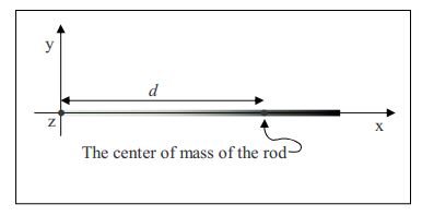
Encuentra el momento de inercia de la varilla a partir de ejemplos\(\ref{22-1}\) and \(\ref{22-2}\), with respect to an axis that is perpendicular to the rod and passes through the center of mass of the rod.

Solution

Recall that the rod in question extends along the \(x\) axis from \(x=0\) to \(x=L\) with \(L=0.890 m\) and that the rod has a linear density given by \(\mu=bL^2\) with \(b=0.650 \frac{kg}{m^3} x^2\).

The axis in question can be chosen to be one that is parallel to the z axis, the axis about which, in solving example \(\ref{22-2}\), we found the moment of inertia to be \(I=0.0726kg \cdot m^2\). In solving example \(\ref{22-1}\) we found the mass of the rod to be \(m=0.1527 kg\) and the center of mass of the rod to be at a distance \(d=0.668 m\) away from the z axis. Here we present the solution to the problem:

\[I=I_{cm}+md^2 \]

\[I_{cm}=I-md^2\]

\[I_{cm}=0.0726kg\cdot m^2-0.1527kg (0.668m)^2\]

\[I_{cm}=0.0047 kg\cdot m^2\]