8.4: Funciones de distribución

8.4.1 Funciones de distribución de una partícula

¿Cuál es el número medio de partículas en la caja de volumen d ³ r _A sobre r _A?

La probabilidad de que la partícula 1 esté en d ³ r _A aproximadamente r _A es

\[ \frac{d^{3} r_{A} \int d^{3} r_{2} \int d^{3} r_{3} \cdots \int d^{3} r_{N} \int d^{3} p_{1} \cdots \int d^{3} p_{N} e^{-\beta H\left(\mathbf{r}_{A}, \mathbf{r}_{2}, \mathbf{r}_{3}, \ldots, \mathbf{r}_{N}, \mathbf{p}_{1}, \ldots, \mathbf{p}_{N}\right)}}{\int d^{3} r_{1} \int d^{3} r_{2} \int d^{3} r_{3} \cdots \int d^{3} r_{N} \int d^{3} p_{1} \cdots \int d^{3} p_{N} e^{-\beta H\left(\mathbf{r}_{1}, \mathbf{r}_{2}, \mathbf{r}_{3}, \ldots, \mathbf{r}_{N}, \mathbf{p}_{1}, \ldots, \mathbf{p}_{N}\right)}}.\]

La probabilidad de que la partícula 2 esté en d ³ r _A aproximadamente r _A es

\[ \frac{\int d^{3} r_{1} \quad d^{3} r_{A} \int d^{3} r_{3} \cdots \int d^{3} r_{N} \int d^{3} p_{1} \cdots \int d^{3} p_{N} e^{-\beta H\left(\mathbf{r}_{1}, \mathbf{r}_{A}, r_{3}, \ldots, \mathbf{r}_{N}, \mathbf{p}_{1}, \ldots, \mathbf{p}_{N}\right)}}{\int d^{3} r_{1} \int d^{3} r_{2} \int d^{3} r_{3} \cdots \int d^{3} r_{N} \int d^{3} p_{1} \cdots \int d^{3} p_{N} e^{-\beta H\left(\mathbf{r}_{1}, \mathbf{r}_{2}, r_{3}, \ldots, \mathbf{r}_{N}, \mathbf{p}_{1}, \ldots, \mathbf{p}_{N}\right)}}.\]

Y así sucesivamente. Podría anotar N integrales diferentes, pero todas serían iguales.

Así, el número medio de partículas en d ³ r _A aproximadamente r _A es

\( \pi_{1}\left(\mathbf{r}_{A}\right) d^{3} \boldsymbol{T}_{A}\)

\[ =N \frac{d^{3} r_{A} \int d^{3} r_{2} \int d^{3} r_{3} \cdots \int d^{3} r_{N} \int d^{3} p_{1} \cdots \int d^{3} p_{N} e^{-\beta H\left(\mathbf{r}_{A}, \mathbf{r}_{2}, \mathbf{r}_{3}, \ldots, \mathbf{r}_{N}, \mathbf{p}_{1}, \ldots, \mathbf{p}_{N}\right)}}{\int d^{3} r_{1} \int d^{3} r_{2} \int d^{3} r_{3} \cdots \int d^{3} r_{N} \int d^{3} p_{1} \cdots \int d^{3} p_{N} e^{-\beta H\left(\mathbf{r}_{1}, \mathbf{r}_{2}, \mathbf{r}_{3}, \ldots, \mathbf{r}_{N}, \mathbf{p}_{1}, \ldots, \mathbf{p}_{N}\right)}}\]

\[ =N \frac{d^{3} r_{A} \int d^{3} r_{2} \int d^{3} r_{3} \cdots \int d^{3} r_{N} \int d^{3} p_{1} \cdots \int d^{3} p_{N} e^{-\beta H\left(\mathbf{r}_{A}, r_{2}, r_{3}, \ldots, r_{N}, \mathbf{p}_{1}, \ldots, \mathbf{p}_{N}\right)}}{h^{3 N} N ! Z(T, V, N)}\]

\[ =\frac{1}{(N-1) !} \frac{d^{3} r_{A} \int d^{3} r_{2} \int d^{3} r_{3} \cdots \int d^{3} r_{N} e^{-\beta U\left(r_{A}, r_{2}, r_{3}, \ldots, r_{N}\right)}}{Q(T, V, N)}\]

8.4.2 Funciones de distribución de dos partículas

Cuál es el número medio de pares de partículas, tal que un miembro del par en una caja de volumen d ³ r _A aproximadamente r _A y el otro miembro está en una caja de volumen d ³ r _B sobre r _B?

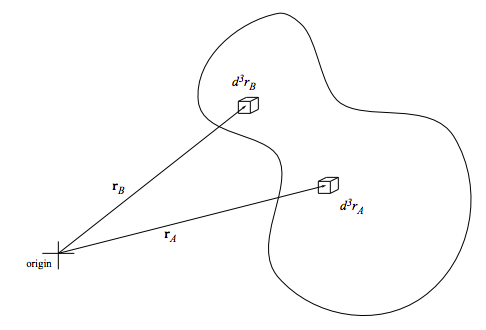
La probabilidad de que la partícula 1 esté en d ³ r _A aproximadamente r _A y la partícula 2 esté en d ³ r _B aproximadamente r _B es

\[ \frac{d^{3} r_{A}}{\int d^{3} r_{1} \int d^{3} r_{2} \int d^{3} r_{3} \cdots \int d^{3} r_{N} \int d^{3} p_{1} \cdots \int d^{3} p_{N} e^{-\beta H\left(\mathbf{r}_{A}, \mathbf{r}_{B}, \mathbf{r}_{3}, \ldots, \mathbf{r}_{N}, \mathbf{p}_{1}, \ldots, \mathbf{p}_{N}\right)}}.\]

La probabilidad de que la partícula 2 esté en d ³ r _A aproximadamente r _A y la partícula 1 esté en d ³ r _B aproximadamente r _B es

\[ \frac{d^{3} r_{B} d^{3} r_{A} \int d^{3} r_{3} \cdots \int d^{3} r_{N} \int d^{3} p_{1} \cdots \int d^{3} p_{N} e^{-\beta H\left(\mathbf{r}_{B}, r_{A}, r_{3}, \ldots, r_{N}, \mathbf{p}_{1}, \ldots, \mathbf{p}_{N}\right)}}{\int d^{3} r_{1} \int d^{3} r_{2} \int d^{3} r_{3} \cdots \int d^{3} r_{N} \int d^{3} p_{1} \cdots \int d^{3} p_{N} e^{-\beta H\left(\mathbf{r}_{1}, \mathbf{r}_{2}, r_{3}, \ldots, \mathbf{r}_{N}, \mathbf{p}_{1}, \ldots, \mathbf{p}_{N}\right)}}.\]

La probabilidad de que la partícula 3 esté en ³ r _A aproximadamente r _A y la partícula 1 esté en d ³ r _B aproximadamente r _B es

\[ \frac{d^{3} r_{B} \int d^{3} r_{2} d^{3} r_{A} \cdots \int d^{3} r_{N} \int d^{3} p_{1} \cdots \int d^{3} p_{N} e^{-\beta H\left(\mathbf{r}_{B}, \mathbf{r}_{2}, r_{A}, \ldots, \mathbf{r}_{N}, \mathbf{p}_{1}, \ldots, \mathbf{p}_{N}\right)}}{\int d^{3} r_{1} \int d^{3} r_{2} \int d^{3} r_{3} \cdots \int d^{3} r_{N} \int d^{3} p_{1} \cdots \int d^{3} p_{N} e^{-\beta H\left(\mathbf{r}_{1}, \mathbf{r}_{2}, r_{3}, \ldots, \mathbf{r}_{N}, \mathbf{p}_{1}, \ldots, \mathbf{p}_{N}\right)}}.\]

Y así sucesivamente. Podría anotar N (N − 1) diferentes integrales, pero todas serían iguales.

Así, el número medio de pares con una partícula en d ³ r _A aproximadamente r _A y la otra en d ³ r _B aproximadamente r _B es

\( n_{2}\left(\mathbf{r}_{A}, \mathbf{r}_{B}\right) d^{3} r_{A} d^{3} r_{B}\)

\[ =N(N-1) \frac{d^{3} r_{A} d^{3} r_{B} \int d^{3} r_{3} \cdots \int d^{3} r_{N} \int d^{3} p_{1} \cdots \int d^{3} p_{N} e^{-\beta H\left(\mathbf{r}_{A}, \mathbf{r}_{B}, \mathbf{r}_{3}, \ldots, \mathbf{r}_{N}, \mathbf{p}_{1}, \ldots, \mathbf{p}_{N}\right)}}{\int d^{3} r_{1} \int d^{3} r_{2} \int d^{3} r_{3} \cdots \int d^{3} r_{N} \int d^{3} p_{1} \cdots \int d^{3} p_{N} e^{-\beta H\left(\mathbf{r}_{1}, \mathbf{r}_{2}, \mathbf{r}_{3}, \ldots, \mathbf{r}_{N}, \mathbf{p}_{1}, \ldots, \mathbf{p}_{N}\right)}}\]

\[ =\frac{1}{(N-2) !} \frac{d^{3} r_{A} d^{3} r_{B} \int d^{3} r_{3} \cdots \int d^{3} r_{N} e^{-\beta U\left(\mathbf{r}_{A}, \mathbf{r}_{B}, \mathbf{r}_{3}, \ldots, \mathbf{r}_{N}\right)}}{Q(T, V, N)}.\]

Problemas

8.7 Correlaciones de partículas cercanas

Supongamos que (como es habitual) a pequeñas distancias el potencial interatómico u (r) es altamente repulsivo. Argumentan que a pequeña r,

\[ g_{2}(r) \approx \text { constant } e^{-u(r) / k_{B} T}.\]

No anotar una derivación larga o elaborada. Busco un simple argumento cualitativo.

8.8 Correlaciones entre partículas cuánticas idénticas que no interactúan

Adivina la forma de la función de correlación de pares g ₂ (r) para fermiones y bosones ideales (no interaccionantes). Esboza tus conjeturas y luego compárelas con las gráficas presentadas por G. Baym en Conferencias sobre Mecánica Cuántica (W.A. Benjamin, Inc., Reading, Mass., 1969) páginas 428 y 431.

8.9 Funciones de correlación y factores de estructura

Un fluido isotrópico típico, a temperaturas superiores a la temperatura crítica, tiene funciones de correlación que son complicadas a distancias cortas, pero que caen exponencialmente a largas distancias. De hecho, el comportamiento a larga distancia es

\[ g_{2}(r)=1+\frac{A e^{-r / \xi}}{r}\]

donde, la llamada longitud de correlación, depende de la temperatura y la densidad. Por el contrario, a la temperatura crítica la función de correlación disminuye mucho más lentamente, ya que

\[ g_{2}(r)=1+\frac{A}{r^{1+\eta}}\]

Encuentra el factor de estructura

\[ S(\mathbf{k})=\int d^{3} r\left[g_{2}(\mathbf{r})-1\right] e^{-i \mathbf{k} \cdot \mathbf{r}}\]

asociados con cada una de estas funciones de correlación. ¿Sus resultados coincidirán con los de los experimentos a valores pequeños de k o a valores grandes (es decir, a longitudes de onda largas o cortas)?

8.10 Factor de estructura de longitud de onda larga

Mostrar que, para un fluido isotrópico,\( \frac{d S(k)}{d k}\) desaparece a k = 0. Aquí S (k) es el factor de estructura

\[ S(\mathbf{k})=1+\rho \int d^{3} r\left[g_{2}(\mathbf{r})-1\right] e^{i \mathbf{k} \cdot \mathbf{r}}.\]

8.11 Correlaciones en un sistema magnético

En el modelo Ising para un imán, descrito en el problema 4.9, la función de correlación (neta) se define por

\[ G_{i} \equiv\left\langle s_{0} s_{i}\right\rangle-\left\langle s_{0}\right\rangle^{2},\]

donde el sitio j = 0 es algún “giro central” arbitrario. Utilizando los resultados del problema 4.9, muestran que para una celosía de N sitios,

\[ \chi_{T}(T, H)=N \frac{m^{2}}{k_{B} T} \sum_{i} G_{i}.\]