
2.8: Formas de pulso y productos de ancho de banda de tiempo
- Page ID
- 84834

La siguiente tabla 2.2 muestra los productos de forma de pulso, espectro y ancho de banda de tiempo de algunas formas de pulso de uso frecuente.
| \(a(t)\) | \(\hat{a} (\omega) = \int_{-\infty}^{\infty} a(t) e^{-j\omega t} dt\) | \(\Delta t\) | \(\Delta t \cdot \Delta f\) |
|---|---|---|---|
| \ (a (t)\) ">Gauss:\(e^{-\tfrac{t^2}{t\tau^2}}\) | \ (\ hat {a} (\ omega) =\ int_ {-\ infty} ^ {\ infty} a (t) e^ {-j\ omega t} dt\) ">\(\sqrt{2\pi} \tau e^{-\tfrac{1}{t} \tau^2 \omega^2}\) | \ (\ Delta t\) ">\(2\sqrt{\ln 2} \tau\) | \ (\ Delta t\ cdot\ Delta f\) ">0.441 |
| \ (a (t)\) ">
Hiperbolicecante: sech (\(\dfrac{t}{\tau}\)) |
\ (\ hat {a} (\ omega) =\ int_ {-\ infty} ^ {\ infty} a (t) e^ {-j\ omega t} dt\) ">\(\dfrac{\tau}{2}\) sech (\(\dfrac{\pi}{2} \tau \omega\)) | \ (\ Delta t\) ">\(1.7627 \tau\) | \ (\ Delta t\ cdot\ Delta f\) ">0.315 |
| \ (a (t)\) ">Función rect: \(= \begin{cases} 1, |t| \le \tau/2 \\ 0, |t| > \tau/2 \end{cases}\) |
\ (\ hat {a} (\ omega) =\ int_ {-\ infty} ^ {\ infty} a (t) e^ {-j\ omega t} dt\) ">\(\tau \dfrac{\sin (\tau \omega/2)}{\tau \omega/2}\) | \ (\ Delta t\) ">\(\tau\) | \ (\ Delta t\ cdot\ Delta f\) ">0.886 |
| \ (a (t)\) ">Lorentziano:\(\dfrac{1}{1 + (t/\tau)^2\) | \ (\ hat {a} (\ omega) =\ int_ {-\ infty} ^ {\ infty} a (t) e^ {-j\ omega t} dt\) ">\(2\pi \tau e^{-|\tau \omega|}\) | \ (\ Delta t\) ">\(1.287 \tau\) | \ (\ Delta t\ cdot\ Delta f\) ">0.142 |
| \ (a (t)\) ">Doble exponencial:\(e^{-|\tfrac{t}{\tau}|}\) | \ (\ hat {a} (\ omega) =\ int_ {-\ infty} ^ {\ infty} a (t) e^ {-j\ omega t} dt\) ">\(\dfrac{\tau}{1 + (\omega \tau)^2}\) | \ (\ Delta t\) ">\(\ln 2 \tau\) | \ (\ Delta t\ cdot\ Delta f\) ">0.142 |
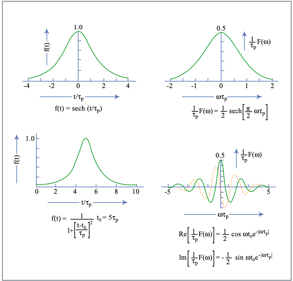
Figura 2.14: Relación de Fourier con la tabla anterior.
Figura por MIT OCW.
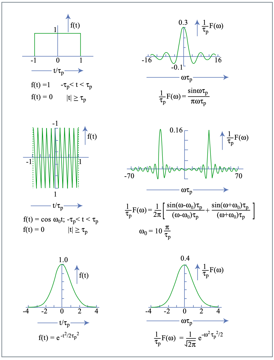
Figura 2.15: Relaciones de Fourier con la tabla anterior. Figura por MIT OCW.
Bibliografía
[1] I. I. Rabi: “Cuantización espacial en un Campo Magnético Giratorio”,. Phys. Rev. 51, 652-654 (1937).
[2] B. R. Mollow, “Espectro de potencia de la luz dispersada por sistemas de dos niveles”, Phys. Rev 188, 1969-1975 (1969).
[3] P. Meystre, M. Sargent III: Elementos de la Óptica Cuántica, Springer Verlag (1990).
[4] L. Allen y J. H. Eberly: Resonancia óptica y átomos de dos niveles, Dover Verlag (1987).
[5] G. B. Whitham: “Ondas lineales y no lineales”, John Wiley and Sons, NY (1973).