
2.7: Ejercicios
- Page ID
- 83398

\( \newcommand{\vecs}[1]{\overset { \scriptstyle \rightharpoonup} {\mathbf{#1}} } \)
\( \newcommand{\vecd}[1]{\overset{-\!-\!\rightharpoonup}{\vphantom{a}\smash {#1}}} \)
\( \newcommand{\id}{\mathrm{id}}\) \( \newcommand{\Span}{\mathrm{span}}\)
( \newcommand{\kernel}{\mathrm{null}\,}\) \( \newcommand{\range}{\mathrm{range}\,}\)
\( \newcommand{\RealPart}{\mathrm{Re}}\) \( \newcommand{\ImaginaryPart}{\mathrm{Im}}\)
\( \newcommand{\Argument}{\mathrm{Arg}}\) \( \newcommand{\norm}[1]{\| #1 \|}\)
\( \newcommand{\inner}[2]{\langle #1, #2 \rangle}\)
\( \newcommand{\Span}{\mathrm{span}}\)
\( \newcommand{\id}{\mathrm{id}}\)
\( \newcommand{\Span}{\mathrm{span}}\)
\( \newcommand{\kernel}{\mathrm{null}\,}\)
\( \newcommand{\range}{\mathrm{range}\,}\)
\( \newcommand{\RealPart}{\mathrm{Re}}\)
\( \newcommand{\ImaginaryPart}{\mathrm{Im}}\)
\( \newcommand{\Argument}{\mathrm{Arg}}\)
\( \newcommand{\norm}[1]{\| #1 \|}\)
\( \newcommand{\inner}[2]{\langle #1, #2 \rangle}\)
\( \newcommand{\Span}{\mathrm{span}}\) \( \newcommand{\AA}{\unicode[.8,0]{x212B}}\)
\( \newcommand{\vectorA}[1]{\vec{#1}} % arrow\)
\( \newcommand{\vectorAt}[1]{\vec{\text{#1}}} % arrow\)
\( \newcommand{\vectorB}[1]{\overset { \scriptstyle \rightharpoonup} {\mathbf{#1}} } \)
\( \newcommand{\vectorC}[1]{\textbf{#1}} \)
\( \newcommand{\vectorD}[1]{\overrightarrow{#1}} \)
\( \newcommand{\vectorDt}[1]{\overrightarrow{\text{#1}}} \)
\( \newcommand{\vectE}[1]{\overset{-\!-\!\rightharpoonup}{\vphantom{a}\smash{\mathbf {#1}}}} \)
\( \newcommand{\vecs}[1]{\overset { \scriptstyle \rightharpoonup} {\mathbf{#1}} } \)
\( \newcommand{\vecd}[1]{\overset{-\!-\!\rightharpoonup}{\vphantom{a}\smash {#1}}} \)
\(\newcommand{\avec}{\mathbf a}\) \(\newcommand{\bvec}{\mathbf b}\) \(\newcommand{\cvec}{\mathbf c}\) \(\newcommand{\dvec}{\mathbf d}\) \(\newcommand{\dtil}{\widetilde{\mathbf d}}\) \(\newcommand{\evec}{\mathbf e}\) \(\newcommand{\fvec}{\mathbf f}\) \(\newcommand{\nvec}{\mathbf n}\) \(\newcommand{\pvec}{\mathbf p}\) \(\newcommand{\qvec}{\mathbf q}\) \(\newcommand{\svec}{\mathbf s}\) \(\newcommand{\tvec}{\mathbf t}\) \(\newcommand{\uvec}{\mathbf u}\) \(\newcommand{\vvec}{\mathbf v}\) \(\newcommand{\wvec}{\mathbf w}\) \(\newcommand{\xvec}{\mathbf x}\) \(\newcommand{\yvec}{\mathbf y}\) \(\newcommand{\zvec}{\mathbf z}\) \(\newcommand{\rvec}{\mathbf r}\) \(\newcommand{\mvec}{\mathbf m}\) \(\newcommand{\zerovec}{\mathbf 0}\) \(\newcommand{\onevec}{\mathbf 1}\) \(\newcommand{\real}{\mathbb R}\) \(\newcommand{\twovec}[2]{\left[\begin{array}{r}#1 \\ #2 \end{array}\right]}\) \(\newcommand{\ctwovec}[2]{\left[\begin{array}{c}#1 \\ #2 \end{array}\right]}\) \(\newcommand{\threevec}[3]{\left[\begin{array}{r}#1 \\ #2 \\ #3 \end{array}\right]}\) \(\newcommand{\cthreevec}[3]{\left[\begin{array}{c}#1 \\ #2 \\ #3 \end{array}\right]}\) \(\newcommand{\fourvec}[4]{\left[\begin{array}{r}#1 \\ #2 \\ #3 \\ #4 \end{array}\right]}\) \(\newcommand{\cfourvec}[4]{\left[\begin{array}{c}#1 \\ #2 \\ #3 \\ #4 \end{array}\right]}\) \(\newcommand{\fivevec}[5]{\left[\begin{array}{r}#1 \\ #2 \\ #3 \\ #4 \\ #5 \\ \end{array}\right]}\) \(\newcommand{\cfivevec}[5]{\left[\begin{array}{c}#1 \\ #2 \\ #3 \\ #4 \\ #5 \\ \end{array}\right]}\) \(\newcommand{\mattwo}[4]{\left[\begin{array}{rr}#1 \amp #2 \\ #3 \amp #4 \\ \end{array}\right]}\) \(\newcommand{\laspan}[1]{\text{Span}\{#1\}}\) \(\newcommand{\bcal}{\cal B}\) \(\newcommand{\ccal}{\cal C}\) \(\newcommand{\scal}{\cal S}\) \(\newcommand{\wcal}{\cal W}\) \(\newcommand{\ecal}{\cal E}\) \(\newcommand{\coords}[2]{\left\{#1\right\}_{#2}}\) \(\newcommand{\gray}[1]{\color{gray}{#1}}\) \(\newcommand{\lgray}[1]{\color{lightgray}{#1}}\) \(\newcommand{\rank}{\operatorname{rank}}\) \(\newcommand{\row}{\text{Row}}\) \(\newcommand{\col}{\text{Col}}\) \(\renewcommand{\row}{\text{Row}}\) \(\newcommand{\nul}{\text{Nul}}\) \(\newcommand{\var}{\text{Var}}\) \(\newcommand{\corr}{\text{corr}}\) \(\newcommand{\len}[1]{\left|#1\right|}\) \(\newcommand{\bbar}{\overline{\bvec}}\) \(\newcommand{\bhat}{\widehat{\bvec}}\) \(\newcommand{\bperp}{\bvec^\perp}\) \(\newcommand{\xhat}{\widehat{\xvec}}\) \(\newcommand{\vhat}{\widehat{\vvec}}\) \(\newcommand{\uhat}{\widehat{\uvec}}\) \(\newcommand{\what}{\widehat{\wvec}}\) \(\newcommand{\Sighat}{\widehat{\Sigma}}\) \(\newcommand{\lt}{<}\) \(\newcommand{\gt}{>}\) \(\newcommand{\amp}{&}\) \(\definecolor{fillinmathshade}{gray}{0.9}\)(Supongamos que los diodos son silicio a menos que se indique
2.7.1: Problemas de análisis
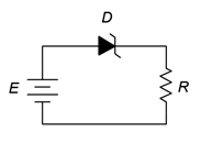
1. Para el circuito de la Figura\(\PageIndex{1}\) determinar la corriente circulante si el suministro es de 6 voltios y la resistencia es de 10 k\(\Omega\).
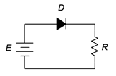
Figura\(\PageIndex{1}\)
2. Repita el problema 1 si el diodo se inserta en la orientación opuesta.
3. Dado el circuito de la Figura\(\PageIndex{2}\), determinar las caídas de voltaje a través de las resistencias. La fuente es de 12 voltios,\(R_1\) = 4.7 k y\(R_2\) = 3.3 k.
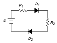
Figura\(\PageIndex{2}\)
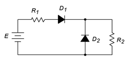
4. En la Figura\(\PageIndex{3}\) determinar las caídas de voltaje a través de las resistencias.
Figura\(\PageIndex{3}\)
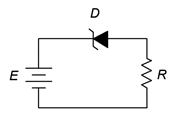
5. Determine la corriente del LED en la Figura\(\PageIndex{4}\). Supongamos que la barrera LED es de 2.1 voltios, la fuente es de 5 voltios y la resistencia es 330\(\Omega\).
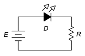
Figura\(\PageIndex{4}\)
6. Repita el problema 5 si el LED está insertado en orientación inversa.
7. Determine las corrientes de resistencia en la Figura\(\PageIndex{5}\). La fuente es de 15 voltios,\(R_1\) = 8.2 k y\(R_2\) = 3.9 k.
Figura\(\PageIndex{5}\)
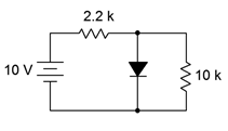
8. Para el circuito de la Figura\(\PageIndex{6}\), determine el voltaje de la resistencia. La fuente es de 9 voltios, el potencial Zener es de 5.1 voltios y la resistencia es de 1 k.
Figura\(\PageIndex{6}\)
9. Para el circuito de la Figura\(\PageIndex{7}\), determine el voltaje de la resistencia. La fuente es de 8 voltios, el potencial Zener es de 3.3 voltios y la resistencia es de 10 k.
Figura\(\PageIndex{7}\)
10. Determine el voltaje\(R_2\) en la Figura\(\PageIndex{8}\) si la fuente es de 9 voltios, el Zener es 6.8 voltios,\(R_1\) = 5.1 k y\(R_2\) = 33 k.
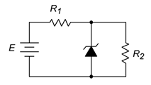
Figura\(\PageIndex{8}\)
2.7.2: Problemas de desafío
11. Determine el voltaje de la resistencia en la Figura\(\PageIndex{9}\) si\(E_1\) = 5 voltios,\(E_2\) = 9 voltios y\(R\) = 1 k.
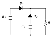
Figura\(\PageIndex{9}\)
12. Determine el voltaje\(R_2\) en la Figura\(\PageIndex{8}\) si la fuente es de 9 voltios, el Zener es 5.6 voltios,\(R_1\) = 5.1 k y\(R_2\) = 3.9 k.
2.7.3: Problemas de diseño
13. Determine un valor para\(R\) en la Figura\(\PageIndex{1}\) para establecer la corriente a 10 mA si la fuente es de 5 voltios.
14. Determine un valor para\(R\) en la Figura\(\PageIndex{4}\) que establecerá la corriente del LED en aproximadamente 20 mA si la fuente es de 9 voltios y el LED es de tipo rojo estándar. Utilice un valor de resistencia estándar.
2.7.4: Problemas de simulación por computadora
15. Simular Problema 9.
16. Simular el circuito diseñado en el Problema 14 para su verificación.