
6.7: Ejercicios
- Page ID
- 83431

\( \newcommand{\vecs}[1]{\overset { \scriptstyle \rightharpoonup} {\mathbf{#1}} } \)
\( \newcommand{\vecd}[1]{\overset{-\!-\!\rightharpoonup}{\vphantom{a}\smash {#1}}} \)
\( \newcommand{\id}{\mathrm{id}}\) \( \newcommand{\Span}{\mathrm{span}}\)
( \newcommand{\kernel}{\mathrm{null}\,}\) \( \newcommand{\range}{\mathrm{range}\,}\)
\( \newcommand{\RealPart}{\mathrm{Re}}\) \( \newcommand{\ImaginaryPart}{\mathrm{Im}}\)
\( \newcommand{\Argument}{\mathrm{Arg}}\) \( \newcommand{\norm}[1]{\| #1 \|}\)
\( \newcommand{\inner}[2]{\langle #1, #2 \rangle}\)
\( \newcommand{\Span}{\mathrm{span}}\)
\( \newcommand{\id}{\mathrm{id}}\)
\( \newcommand{\Span}{\mathrm{span}}\)
\( \newcommand{\kernel}{\mathrm{null}\,}\)
\( \newcommand{\range}{\mathrm{range}\,}\)
\( \newcommand{\RealPart}{\mathrm{Re}}\)
\( \newcommand{\ImaginaryPart}{\mathrm{Im}}\)
\( \newcommand{\Argument}{\mathrm{Arg}}\)
\( \newcommand{\norm}[1]{\| #1 \|}\)
\( \newcommand{\inner}[2]{\langle #1, #2 \rangle}\)
\( \newcommand{\Span}{\mathrm{span}}\) \( \newcommand{\AA}{\unicode[.8,0]{x212B}}\)
\( \newcommand{\vectorA}[1]{\vec{#1}} % arrow\)
\( \newcommand{\vectorAt}[1]{\vec{\text{#1}}} % arrow\)
\( \newcommand{\vectorB}[1]{\overset { \scriptstyle \rightharpoonup} {\mathbf{#1}} } \)
\( \newcommand{\vectorC}[1]{\textbf{#1}} \)
\( \newcommand{\vectorD}[1]{\overrightarrow{#1}} \)
\( \newcommand{\vectorDt}[1]{\overrightarrow{\text{#1}}} \)
\( \newcommand{\vectE}[1]{\overset{-\!-\!\rightharpoonup}{\vphantom{a}\smash{\mathbf {#1}}}} \)
\( \newcommand{\vecs}[1]{\overset { \scriptstyle \rightharpoonup} {\mathbf{#1}} } \)
\( \newcommand{\vecd}[1]{\overset{-\!-\!\rightharpoonup}{\vphantom{a}\smash {#1}}} \)
\(\newcommand{\avec}{\mathbf a}\) \(\newcommand{\bvec}{\mathbf b}\) \(\newcommand{\cvec}{\mathbf c}\) \(\newcommand{\dvec}{\mathbf d}\) \(\newcommand{\dtil}{\widetilde{\mathbf d}}\) \(\newcommand{\evec}{\mathbf e}\) \(\newcommand{\fvec}{\mathbf f}\) \(\newcommand{\nvec}{\mathbf n}\) \(\newcommand{\pvec}{\mathbf p}\) \(\newcommand{\qvec}{\mathbf q}\) \(\newcommand{\svec}{\mathbf s}\) \(\newcommand{\tvec}{\mathbf t}\) \(\newcommand{\uvec}{\mathbf u}\) \(\newcommand{\vvec}{\mathbf v}\) \(\newcommand{\wvec}{\mathbf w}\) \(\newcommand{\xvec}{\mathbf x}\) \(\newcommand{\yvec}{\mathbf y}\) \(\newcommand{\zvec}{\mathbf z}\) \(\newcommand{\rvec}{\mathbf r}\) \(\newcommand{\mvec}{\mathbf m}\) \(\newcommand{\zerovec}{\mathbf 0}\) \(\newcommand{\onevec}{\mathbf 1}\) \(\newcommand{\real}{\mathbb R}\) \(\newcommand{\twovec}[2]{\left[\begin{array}{r}#1 \\ #2 \end{array}\right]}\) \(\newcommand{\ctwovec}[2]{\left[\begin{array}{c}#1 \\ #2 \end{array}\right]}\) \(\newcommand{\threevec}[3]{\left[\begin{array}{r}#1 \\ #2 \\ #3 \end{array}\right]}\) \(\newcommand{\cthreevec}[3]{\left[\begin{array}{c}#1 \\ #2 \\ #3 \end{array}\right]}\) \(\newcommand{\fourvec}[4]{\left[\begin{array}{r}#1 \\ #2 \\ #3 \\ #4 \end{array}\right]}\) \(\newcommand{\cfourvec}[4]{\left[\begin{array}{c}#1 \\ #2 \\ #3 \\ #4 \end{array}\right]}\) \(\newcommand{\fivevec}[5]{\left[\begin{array}{r}#1 \\ #2 \\ #3 \\ #4 \\ #5 \\ \end{array}\right]}\) \(\newcommand{\cfivevec}[5]{\left[\begin{array}{c}#1 \\ #2 \\ #3 \\ #4 \\ #5 \\ \end{array}\right]}\) \(\newcommand{\mattwo}[4]{\left[\begin{array}{rr}#1 \amp #2 \\ #3 \amp #4 \\ \end{array}\right]}\) \(\newcommand{\laspan}[1]{\text{Span}\{#1\}}\) \(\newcommand{\bcal}{\cal B}\) \(\newcommand{\ccal}{\cal C}\) \(\newcommand{\scal}{\cal S}\) \(\newcommand{\wcal}{\cal W}\) \(\newcommand{\ecal}{\cal E}\) \(\newcommand{\coords}[2]{\left\{#1\right\}_{#2}}\) \(\newcommand{\gray}[1]{\color{gray}{#1}}\) \(\newcommand{\lgray}[1]{\color{lightgray}{#1}}\) \(\newcommand{\rank}{\operatorname{rank}}\) \(\newcommand{\row}{\text{Row}}\) \(\newcommand{\col}{\text{Col}}\) \(\renewcommand{\row}{\text{Row}}\) \(\newcommand{\nul}{\text{Nul}}\) \(\newcommand{\var}{\text{Var}}\) \(\newcommand{\corr}{\text{corr}}\) \(\newcommand{\len}[1]{\left|#1\right|}\) \(\newcommand{\bbar}{\overline{\bvec}}\) \(\newcommand{\bhat}{\widehat{\bvec}}\) \(\newcommand{\bperp}{\bvec^\perp}\) \(\newcommand{\xhat}{\widehat{\xvec}}\) \(\newcommand{\vhat}{\widehat{\vvec}}\) \(\newcommand{\uhat}{\widehat{\uvec}}\) \(\newcommand{\what}{\widehat{\wvec}}\) \(\newcommand{\Sighat}{\widehat{\Sigma}}\) \(\newcommand{\lt}{<}\) \(\newcommand{\gt}{>}\) \(\newcommand{\amp}{&}\) \(\definecolor{fillinmathshade}{gray}{0.9}\)6.7.1: Problemas de análisis
1. Determinar el voltaje de carga para el modelo de la Figura\(\PageIndex{1}\) if\(V_{gen}\) = 10 mV\(\Omega\),\(Z_{gen}\)\(Z_{in}\) = 50, = 1 M\(\Omega\),\(Z_{out}\) = 75\(\Omega\),\(Z_{load}\) = 1 k\(\Omega\) y\(A_v\) = 50.
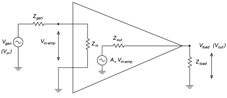
Figura\(\PageIndex{1}\)
2. Determinar el voltaje de carga para el modelo de la Figura\(\PageIndex{1}\) dado\(V_{gen}\) = 8 mV,\(Z_{gen}\) = 1 k\(\Omega\),\(Z_{in}\) = 6 k\(\Omega\),\(Z_{out}\) = 500\(\Omega\),\(Z_{load}\) = 2 k\(\Omega\) y\(A_v\) = 100.
3. Si el circuito del Problema 1 tiene una conformidad de 2 voltios, ¿se acortará la salida? ¿Qué pasa si la entrada se incrementa a 100 mV?
4. Si el circuito del Problema 2 tiene una conformidad de 5 voltios, ¿se acortará la salida? ¿Qué pasa si la entrada se incrementa a 200 mV?
5. Si un amplificador tiene\(A_v\) = 25,\(V_{in}\) = 20 mV y no hay carga apreciable, determine la relación señal/ruido de salida si el amplificador genera una tensión de ruido de salida de 10\(\mu\) V.
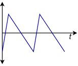
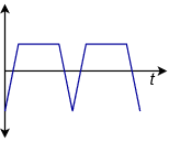
6. Determine qué formas de onda desde las Figuras\(\PageIndex{2}\) hasta\(\PageIndex{6}\) exhiben simetría de media onda.
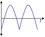
Figura\(\PageIndex{2}\)
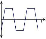
Figura\(\PageIndex{3}\)
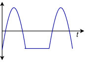
Figura\(\PageIndex{4}\)
Figura\(\PageIndex{5}\)
Figura\(\PageIndex{6}\)
7. Determinar las resistencias equivalentes Miller para el circuito de la Figura\(\PageIndex{7}\) if\(A_v\) = −20 y\(R\) = 60 k\(\Omega\).
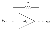
Figura\(\PageIndex{7}\)
8. Determinar las capacitancias equivalentes de Miller para el circuito de la Figura\(\PageIndex{8}\) asumiendo\(A_v\) = −30 y\(C\) = 200 pF.
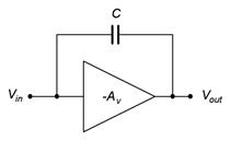
Figura\(\PageIndex{8}\)
6.7.2: Problemas de desafío
9. Si el circuito del Problema 1 tiene una conformidad de 20 voltios, ¿qué tan grande puede ser la señal de entrada antes de que se recorte el voltaje de carga?
10. Si el circuito del Problema 2 tiene una conformidad de 10 voltios, ¿qué tan grande puede ser la señal de entrada antes de que se recorte el voltaje de carga?
11. Usando Figura\(\PageIndex{7}\) como guía y asumiendo que\(R\) = 100 k\(\Omega\), ¿qué tan grande tendría que ser la ganancia tal que la resistencia equivalente de entrada sea de 4 k\(\Omega\)?
12. Usando Figura\(\PageIndex{8}\) como guía y suponiendo que\(A_v\) = −35, determine un valor para\(C\) tal que la capacitancia equivalente de entrada sea 1.2 nF.
6.7.3: Problemas de simulación por computadora
13. Simule el circuito del Problema 1 y verifique el voltaje de carga.
14. Simule el circuito del Problema 2 y verifique el voltaje de carga.