
4.5: Introducción a la Teoría de las Gráficas
- Page ID
- 117110

\( \newcommand{\vecs}[1]{\overset { \scriptstyle \rightharpoonup} {\mathbf{#1}} } \)
\( \newcommand{\vecd}[1]{\overset{-\!-\!\rightharpoonup}{\vphantom{a}\smash {#1}}} \)
\( \newcommand{\dsum}{\displaystyle\sum\limits} \)
\( \newcommand{\dint}{\displaystyle\int\limits} \)
\( \newcommand{\dlim}{\displaystyle\lim\limits} \)
\( \newcommand{\id}{\mathrm{id}}\) \( \newcommand{\Span}{\mathrm{span}}\)
( \newcommand{\kernel}{\mathrm{null}\,}\) \( \newcommand{\range}{\mathrm{range}\,}\)
\( \newcommand{\RealPart}{\mathrm{Re}}\) \( \newcommand{\ImaginaryPart}{\mathrm{Im}}\)
\( \newcommand{\Argument}{\mathrm{Arg}}\) \( \newcommand{\norm}[1]{\| #1 \|}\)
\( \newcommand{\inner}[2]{\langle #1, #2 \rangle}\)
\( \newcommand{\Span}{\mathrm{span}}\)
\( \newcommand{\id}{\mathrm{id}}\)
\( \newcommand{\Span}{\mathrm{span}}\)
\( \newcommand{\kernel}{\mathrm{null}\,}\)
\( \newcommand{\range}{\mathrm{range}\,}\)
\( \newcommand{\RealPart}{\mathrm{Re}}\)
\( \newcommand{\ImaginaryPart}{\mathrm{Im}}\)
\( \newcommand{\Argument}{\mathrm{Arg}}\)
\( \newcommand{\norm}[1]{\| #1 \|}\)
\( \newcommand{\inner}[2]{\langle #1, #2 \rangle}\)
\( \newcommand{\Span}{\mathrm{span}}\) \( \newcommand{\AA}{\unicode[.8,0]{x212B}}\)
\( \newcommand{\vectorA}[1]{\vec{#1}} % arrow\)
\( \newcommand{\vectorAt}[1]{\vec{\text{#1}}} % arrow\)
\( \newcommand{\vectorB}[1]{\overset { \scriptstyle \rightharpoonup} {\mathbf{#1}} } \)
\( \newcommand{\vectorC}[1]{\textbf{#1}} \)
\( \newcommand{\vectorD}[1]{\overrightarrow{#1}} \)
\( \newcommand{\vectorDt}[1]{\overrightarrow{\text{#1}}} \)
\( \newcommand{\vectE}[1]{\overset{-\!-\!\rightharpoonup}{\vphantom{a}\smash{\mathbf {#1}}}} \)
\( \newcommand{\vecs}[1]{\overset { \scriptstyle \rightharpoonup} {\mathbf{#1}} } \)
\(\newcommand{\longvect}{\overrightarrow}\)
\( \newcommand{\vecd}[1]{\overset{-\!-\!\rightharpoonup}{\vphantom{a}\smash {#1}}} \)
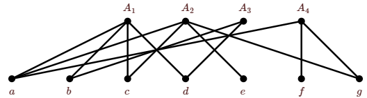
\(\newcommand{\avec}{\mathbf a}\) \(\newcommand{\bvec}{\mathbf b}\) \(\newcommand{\cvec}{\mathbf c}\) \(\newcommand{\dvec}{\mathbf d}\) \(\newcommand{\dtil}{\widetilde{\mathbf d}}\) \(\newcommand{\evec}{\mathbf e}\) \(\newcommand{\fvec}{\mathbf f}\) \(\newcommand{\nvec}{\mathbf n}\) \(\newcommand{\pvec}{\mathbf p}\) \(\newcommand{\qvec}{\mathbf q}\) \(\newcommand{\svec}{\mathbf s}\) \(\newcommand{\tvec}{\mathbf t}\) \(\newcommand{\uvec}{\mathbf u}\) \(\newcommand{\vvec}{\mathbf v}\) \(\newcommand{\wvec}{\mathbf w}\) \(\newcommand{\xvec}{\mathbf x}\) \(\newcommand{\yvec}{\mathbf y}\) \(\newcommand{\zvec}{\mathbf z}\) \(\newcommand{\rvec}{\mathbf r}\) \(\newcommand{\mvec}{\mathbf m}\) \(\newcommand{\zerovec}{\mathbf 0}\) \(\newcommand{\onevec}{\mathbf 1}\) \(\newcommand{\real}{\mathbb R}\) \(\newcommand{\twovec}[2]{\left[\begin{array}{r}#1 \\ #2 \end{array}\right]}\) \(\newcommand{\ctwovec}[2]{\left[\begin{array}{c}#1 \\ #2 \end{array}\right]}\) \(\newcommand{\threevec}[3]{\left[\begin{array}{r}#1 \\ #2 \\ #3 \end{array}\right]}\) \(\newcommand{\cthreevec}[3]{\left[\begin{array}{c}#1 \\ #2 \\ #3 \end{array}\right]}\) \(\newcommand{\fourvec}[4]{\left[\begin{array}{r}#1 \\ #2 \\ #3 \\ #4 \end{array}\right]}\) \(\newcommand{\cfourvec}[4]{\left[\begin{array}{c}#1 \\ #2 \\ #3 \\ #4 \end{array}\right]}\) \(\newcommand{\fivevec}[5]{\left[\begin{array}{r}#1 \\ #2 \\ #3 \\ #4 \\ #5 \\ \end{array}\right]}\) \(\newcommand{\cfivevec}[5]{\left[\begin{array}{c}#1 \\ #2 \\ #3 \\ #4 \\ #5 \\ \end{array}\right]}\) \(\newcommand{\mattwo}[4]{\left[\begin{array}{rr}#1 \amp #2 \\ #3 \amp #4 \\ \end{array}\right]}\) \(\newcommand{\laspan}[1]{\text{Span}\{#1\}}\) \(\newcommand{\bcal}{\cal B}\) \(\newcommand{\ccal}{\cal C}\) \(\newcommand{\scal}{\cal S}\) \(\newcommand{\wcal}{\cal W}\) \(\newcommand{\ecal}{\cal E}\) \(\newcommand{\coords}[2]{\left\{#1\right\}_{#2}}\) \(\newcommand{\gray}[1]{\color{gray}{#1}}\) \(\newcommand{\lgray}[1]{\color{lightgray}{#1}}\) \(\newcommand{\rank}{\operatorname{rank}}\) \(\newcommand{\row}{\text{Row}}\) \(\newcommand{\col}{\text{Col}}\) \(\renewcommand{\row}{\text{Row}}\) \(\newcommand{\nul}{\text{Nul}}\) \(\newcommand{\var}{\text{Var}}\) \(\newcommand{\corr}{\text{corr}}\) \(\newcommand{\len}[1]{\left|#1\right|}\) \(\newcommand{\bbar}{\overline{\bvec}}\) \(\newcommand{\bhat}{\widehat{\bvec}}\) \(\newcommand{\bperp}{\bvec^\perp}\) \(\newcommand{\xhat}{\widehat{\xvec}}\) \(\newcommand{\vhat}{\widehat{\vvec}}\) \(\newcommand{\uhat}{\widehat{\uvec}}\) \(\newcommand{\what}{\widehat{\wvec}}\) \(\newcommand{\Sighat}{\widehat{\Sigma}}\) \(\newcommand{\lt}{<}\) \(\newcommand{\gt}{>}\) \(\newcommand{\amp}{&}\) \(\definecolor{fillinmathshade}{gray}{0.9}\)Podemos interpretar el problema sdr como un problema sobre las gráficas. Dados conjuntos\(A_1,A_2,\ldots,A_n\), con\(\bigcup_{i=1}^n A_i=\{x_1,x_2,\ldots,x_m\}\), definimos una gráfica con\(n+m\) vértices de la siguiente manera: Los vértices están etiquetados\(\{A_1,A_2,\ldots,A_n,x_1,x_2,\ldots x_m\}\), y los bordes son\(\{\{A_i,x_j\}\mid x_j\in A_i\}\).
Ejemplo\(\PageIndex{1}\)
Vamos\(A_1=\{a,b,c,d\}\),\(A_2=\{a,c,e,g\}\),\(A_3=\{b,d\}\), y\(A_4=\{a,f,g\}\). La gráfica correspondiente se muestra en la Figura\(\PageIndex{1}\).
Antes de explorar esta idea, introducimos algunos conceptos básicos sobre las gráficas. Si dos vértices en una gráfica están conectados por un borde, decimos que los vértices son adyacentes. Si un vértice\(v\) es un punto final de borde\(e\), decimos que son incidentes. El conjunto de vértices adyacentes a\(v\) se llama el barrio de\(v\), denotado\(N(v)\). Esto a veces se le llama el barrio abierto de\(v\) para distinguirlo del barrio cerrado de\(v\),\(N[v]=N(v)\cup\{v\}\). El grado de un vértice\(v\) es el número de aristas que inciden con\(v\); se denota\(\text{d}(v)\).
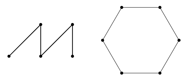
Some simple types of graph come up often: A path is a graph \(P_n\) on vertices \(v_1,v_2,\ldots,v_n\), with edges \(\{v_i,v_{i+1}\}\) for \(1\le i\le n-1\), and no other edges. A cycle is a graph \(C_n\) on vertices \(v_1,v_2,\ldots,v_n\) with edges \(\{v_i,v_{1+(i\bmod n)}\}\) for \(1\le i\le n\), and no other edges; this is a path in which the first and last vertices have been joined by an edge. (Generally, we require that a cycle have at least three vertices. If it has two, then the two are joined by two distinct edges; when a graph has more than one edge with the same endpoints it is called a multigraph. If a cycle has one vertex, there is an edge, called a loop, in which a single vertex serves as both endpoints.) The length of a path or cycle is the number of edges in the graph. For example, \(P_1\) has length 0, \(C_1\) has length 1. A complete graph \(K_n\) is a graph on \(v_1,v_2,\ldots,v_n\) in which every two distinct vertices are joined by an edge. See Figure \(\PageIndex{2}\) for examples.
The graph in Figure \(\PageIndex{1}\) is a bipartite graph.
Definition \(\PageIndex{1}\): Bipartite
A graph \(G\) is bipartite if its vertices can be partitioned into two parts, say \(\{v_1,v_2,\ldots,v_n\}\) and \(\{w_1,w_2,\ldots,w_m\}\) so that all edges join some \(v_i\) to some \(w_j\); no two vertices \(v_i\) and \(v_j\) are adjacent, nor are any vertices \(w_i\) and \(w_j\).
The graph in Figure \(\PageIndex{1}\) is bipartite, as are the first two graphs in Figure \(\PageIndex{2}\).