2.6: RMN H-1 (protón)

Si bien la\(\mathrm{C-} 13\) RMN proporciona información sobre cuántos carbonos químicamente distintos hay en un compuesto, y algo sobre sus entornos electrónicos, no nos dice nada sobre cómo están organizadas las moléculas o qué carbonos están conectados entre sí. ^[18] Para esa información, a menudo recurrimos a la espectroscopia de RMN usando el\(\mathrm{H-} 1\) isótopo. Hay una serie de ventajas para la\(\mathrm{H-} 1\) RMN:\(\mathrm{H-} 1\) es el isótopo natural, más abundante de hidrógeno, y es mucho más abundante que\(\mathrm{C-} 13\). El resultado es que la concentración de\(\mathrm{H-} 1\) en una muestra es mucho mayor que la concentración de\(\mathrm{C-} 13\). Por lo tanto, es más fácil obtener un espectro y se pueden utilizar instrumentos con un campo más bajo. Como veremos, la\(\mathrm{H-} 1\) RMN puede proporcionar información sobre qué átomos están conectados entre sí. Por otro lado, los espectros de\(\mathrm{H-} 1\) RMN resultantes son más complejos.

La teoría básica de ambos\(\mathrm{H-} 1\) y\(\mathrm{C-} 13\) RMN son las mismas y, de hecho, ambos espectros pueden registrarse en un mismo instrumento. La muestra se coloca en un campo magnético que divide los estados de espín de los\(\mathrm{H-} 1\) núcleos; se detecta la energía requerida para voltear los núcleos de un estado de espín a otro y se transforma en un espectro como el de abajo.

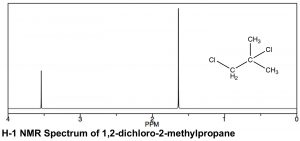
Existen similitudes y diferencias en la apariencia de los\(\mathrm{H-} 1\) espectros de\(\mathrm{C-} 13\) RMN. Como se puede observar en el espectro de 1,2-dicloro-2-metilpropano (\(\leftarrow\)), las escalas sobre las que se registran los espectros son diferentes. Ambos implican un desplazamiento químico de un pico de referencia a 0, (TMS [tetrametilsilano] se usa en ambos), pero el rango de desplazamiento (a menudo referido como\(\delta\), así como\(\mathrm{ppm}\), en RMN protónica) es menor para\(\mathrm{H-} 1\) comparación con\(\mathrm{C-} 13\) RMN. Normalmente se registra un espectro de\(\mathrm{H-} 1\) RMN entre\(0-10 \mathrm{ ppm}\) (a diferencia de\(0-200\) for\(\mathrm{C-} 13\)), aunque en este caso se trunca porque no hay picos entre ellos\(4–10 \mathrm{ ppm}\). Dicho esto, se observan las mismas tendencias en los desplazamientos químicos: cuanto más desblindado están los átomos (en este caso protones), más abajo aparecen. En el espectro de 1,2-dicloro-2-metilpropano anterior hay dos picos correspondientes a los dos tipos de hidrógenos químicamente distintos (es decir, los dos idénticos\(-\mathrm{CH}_{3}\) y el\(\mathrm{-CH}_{2}\) grupo). El campo más bajo del pico, alrededor\(3.6 \mathrm{ ppm}\) puede asignarse al grupo\(\mathrm{CH}_{2}\) (metileno), que está unido directamente al átomo de cloro que retira electrones, mientras que el segundo pico, correspondiente a los seis hidrógenos equivalentes de los dos grupos metilo, está más arriba, alrededor\(1.6 \mathrm{ ppm}\).

En un espectro de RMN protónica, el área bajo el pico es proporcional al número de protones que dan lugar a la señal. Al integrar el área bajo el pico, generamos una estimación de los números relativos de hidrógenos que dan lugar a cada señal. En el espectro de 1,2-dicloro-2-metilpropano la relación de las dos áreas de pico es 1:3, lo que respalda nuestra asignación del pico de campo abajo al\(\mathrm{CH}_{2}\) y el pico de campo superior a los dos hidrógenos de metilo equivalentes\(-\mathrm{CH}_{3}\) (seis). Como nota técnica, las señales de\(\mathrm{C-} 13\) RMN no son proporcionales de manera confiable al número de carbonos equivalentes involucrados: dependen del número de\(\mathrm{H}\)'s unidos a ellas y por lo tanto la integración no puede proporcionar una estimación confiable de las proporciones de los tipos de carbono en un compuesto. ^[19]

División Spin-Spin

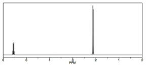
Otra forma en que la\(\mathrm{H-} 1\) RMN difiere de una\(\mathrm{C-} 13\) RMN se muestra en el espectro del 1,1-dicloroetano\(\rightarrow\), que tiene dos tipos de hidrógenos equivalentes. Cada tipo da lugar a una señal distinta pero cada una de esas señales se divide en múltiples picos. La señal de campo superior alrededor\(2 \mathrm{ ppm}\), de los 3 equivalentes\(\mathrm{H}\) del grupo metilo, aparece como un doblete (dos picos separados) porque cada uno de los hidrógenos en el grupo metilo se ve afectado por el campo magnético generado por el posible estado de giro del hidrógeno vecino, alterando así (sumando a o restando de) el campo local de los átomos. La señal de campo abajo alrededor\(5.5 \mathrm{ ppm}\) se debe al protón único encendido\(\mathrm{C-} 1\), desblindado debido a la proximidad del cloro electronegativo, pero ahora aparece como un cuarteto.

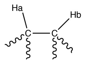
Por ejemplo, considere una molécula que tenga dos protones no equivalentes (\(\mathrm{Ha}\) and \(\mathrm{Hb}\)) on adjacent carbons (\(\rightarrow\)). \(\mathrm{Ha}\) will experience the magnetic fields generated by \(\mathrm{Hb}\) which has two spin states, which will produce two possible electronic environments for \(\mathrm{Ha}\), resulting in two signals for \(\mathrm{Ha}\).

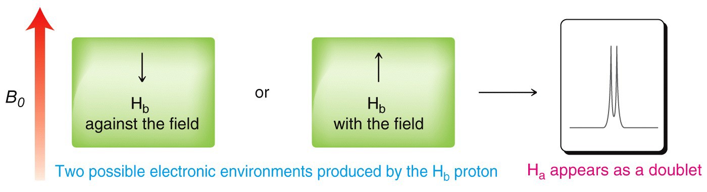
A single proton produces a doublet in the adjacent signal

The splitting effect is small and does not extend (in a significant way) beyond the protons on adjacent carbons. The local magnetic field also depends on the number of protons that do the splitting, for example if there are two protons on the adjacent carbon, the signal is split into a triplet, and for three adjacent protons the signal is a quartet. The general rule is that for \(n\) adjacent protons, the signal is split into \(n+1\) peaks.

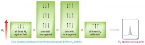
Three adjacent protons produce a quartet in the adjacent signal

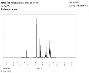
The width, in \(\mathrm{Hz}\), of the splitting (that is, the distance between the split peaks) is called the coupling constant \(j\). The value of \(j\) between the protons on adjacent carbons is the same. The number of split peaks therefore allows us to determine how many hydrogens there are on adjacent carbons, which in turn allows us to determine the how the atoms are connected together in the structure. Signals that are split by more than one kind of hydrogen can get quite messy as shown in the spectrum of D-glucopyranose (\(\rightarrow\)).

Fortunately, there are ways to simplify such spectrum by selectively irradiating particular frequencies but that is beyond the scope of this course (but something you can look forward to in the future!).

That said, this raises another question: why do \(\mathrm{C-} 13\) NMR spectra appear as single lines for each carbon? Shouldn’t the carbon signals also be split both by adjacent carbons, and by the hydrogens attached to them? There are two reasons that this does not happen. First, the abundance of \(\mathrm{C-} 13\) is so low that the probability of finding more than one \(\mathrm{C-} 13\) in a molecule is very low; in the absence of a second (or third) \(\mathrm{C-} 13\), no splitting by adjacent carbon nuclei will occur, (recall \(\mathrm{C-} 12\) does not generate a spin-based magnetic field). Second, when we originally introduced \(\mathrm{C-} 13\) NMR spectroscopy we presented a simplified model. In fact, the carbon signals are split by the adjacent protons, but this leads to a complex spectrum that is often hard to interpret. Therefore, for most purposes, the sample is irradiated with a radiofrequency that promotes all the hydrogens to the higher-energy spin state. The carbon nuclei do not experience two (or more) magnetic field environments, and therefore only one signal is produced. This technique is called broadband decoupling, and these types of spectra are the most common examples of \(\mathrm{C-} 13\) NMR.

Solvents and Acidic hydrogens in the NMR

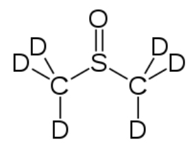
Most NMR spectra, whether \(\mathrm{C-} 13\) or \(\mathrm{H-} 1\), are recorded in solution (although it is possible to obtain spectra on solids—as evidenced by the fact that we can obtain MRI data on people, that say, people [biological systems] are mostly [\(>70 \%\)] water). However, since the solvent is usually present in much greater concentration than the actual sample, as long as we use a solvent that does not generate a strong signal the effects of the solvent can be minimized; typically this involves solvents in which the hydrogens present are replaced with deuterium (D), an isotope of hydrogen that is not NMR active. Common solvents are \(\mathrm{CDCl}_{3}\), (deuterated chloroform) and dimethylsulfoxide \(\mathrm{d-} 6\) (DMSO) (\(\rightarrow\)).

Another instance in which deuterated solvents are used is to detect the presence of potentially acidic hydrogens. Proton transfer is a rapid and reversible process, and any hydrogen attached to an electronegative element is potentially available for exchange by reacting with even very weak base such as water.In fact, by adding a drop of \(\mathrm{D}_{2} \mathrm{O}\) (“heavy” water) to the NMR sample, the signal from any \(\mathrm{O-H}\) or \(\mathrm{N-H}\) disappears as the \(\mathrm{H}\) is replaced by \(\mathrm{D}\).

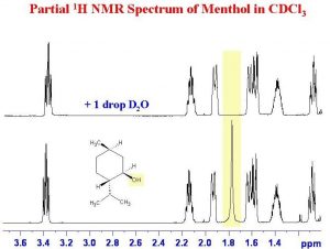
As shown here (\(\rightarrow\)), the signal from the \(\mathrm{OH}\) (shaded in yellow) disappears when the sample is shaken with \(\mathrm{D}_{2} \mathrm{O}\).

Questions to Answer:

Type your exercises here.

• Draw a diagram of an atom and use it to explain why the electron density surrounding the nucleus affects the strength of the external field required to bring the nucleus to resonance (to flip the spin state).
• Using the table below, use your diagram from above and explain a) why the signals for \(\mathrm{C-} 1\) in the three compounds are different, and b) why the signals for \(\mathrm{C-} 1\) and \(\mathrm{C-} 2\) are different (for any single compound).

Compound	Signal for \(\mathrm{C-} 1\)	Signal for \(\mathrm{C-} 1 (\mathrm{ppm})\)
\(\mathrm{CH}_{3} \mathrm{CH}_{2} \mathrm{F}\)	\(\mathrm{C-} 1\)" style="padding:0pt 0pt 0pt 0pt;border:none windowtext 0pt;"> 79.1	\(\mathrm{C-} 1 (\mathrm{ppm})\)" style="padding:0pt 0pt 0pt 0pt;border:none windowtext 0pt;"> 15.4
\(\mathrm{CH}_{3} \mathrm{CH}_{2} \mathrm{Cl}\)	\(\mathrm{C-} 1\)" style="padding:0pt 0pt 0pt 0pt;border:none windowtext 0pt;"> 40.0	\(\mathrm{C-} 1 (\mathrm{ppm})\)" style="padding:0pt 0pt 0pt 0pt;border:none windowtext 0pt;"> 18.9
\(\mathrm{CH}_{3} \mathrm{CH}_{2} \mathrm{Br}\)	\(\mathrm{C-} 1\)" style="padding:0pt 0pt 0pt 0pt;border:none windowtext 0pt;"> 27.5	\(\mathrm{C-} 1 (\mathrm{ppm})\)" style="padding:0pt 0pt 0pt 0pt;border:none windowtext 0pt;"> 19.3