
4.4: Combinaciones de parámetros
- Page ID
- 53158

Antes de avanzar, considere todas las combinaciones posibles de los parámetros, según lo determinado por sus signos. Hay seis posibilidades, ignorando tasas de crecimiento de exactamente cero como infinitamente improbables.
- r>0, s>0 Crecimiento ortólogo.
- r0<0, s> Crecimiento ortólogo con un punto Allee.
- r>0, s=0 Crecimiento exponencial.
- r>0, s<0 Crecimiento logístico con capacidad de carga.
- r<0, s<0 Población inviable decreciendo a la extinción.
- r<0, s=0 Igual que el anterior.
La figura\(\PageIndex{1}\) muestra tres de estas posibilidades ensambladas para formar un modelo poblacional completo. A la izquierda en la figura, número 2 anterior, el crecimiento ortólogo con un punto Allee, prevalece a bajas densidades, donde un mayor número de otros miembros de la especie en las proximidades potencian el crecimiento. En el medio, el número 3 anterior, el crecimiento exponencial, ocurre como una fase de transición. Finalmente a la derecha, número 4 anterior, el crecimiento logístico con capacidad de carga, se hace cargo cuando el hacinamiento y otras limitaciones reducen las tasas de crecimiento a medida que aparecen mayores números de otros miembros de la especie en las cercanías.
El eje vertical de la Figura\(\PageIndex{1}\) muestra la tasa de crecimiento individual, y el eje horizontal muestra la densidad poblacional. A la derecha, donde la pendiente es negativa, a medida que la densidad se acerca − r/s desde la izquierda la tasa de crecimiento en el eje vertical baja a cero, por lo que la población deja de crecer.
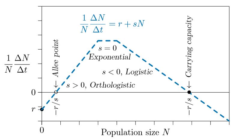
Este es el valor de equilibrio llamado la “capacidad de carga”. Si algo empuja a la población por encima de ese valor —inmigración de animales de otra región, por ejemplo— entonces la tasa de crecimiento en el eje vertical cae por debajo de cero. La tasa de crecimiento es entonces negativa, y por lo tanto la población disminuye. Por otro lado, si algo baja a la población por debajo de ese valor —como la emigración de animales a otro lugar—la tasa de crecimiento en el eje vertical se eleva por encima de cero. Esa tasa de crecimiento es positiva, y por lo tanto la población crece.
La capacidad de carga es “estable”. Se dice que un valor es estable si tiende a restaurarse a sí mismo cuando es empujado por alguna fuerza externa.
 La situación es completamente diferente a la izquierda en la figura, donde la pendiente es positiva. Al igual que a la derecha, cuando la densidad es − r/s, la tasa de crecimiento en el eje vertical llega a cero, es decir, la población no cambia. Esto también es un equilibrio, no una capacidad de carga, sino un punto Allee. Sin embargo, si la población aquí deriva por debajo de − r/s, la tasa de crecimiento en el eje vertical se vuelve negativa y la población disminuye aún más. Es inestable. En este modelo la población continúa disminuyendo hasta su eventual extinción. Por encima del punto Allee, sin embargo, la tasa de crecimiento en el eje vertical es positiva, por lo que la población aumenta hasta alcanzar alguna otra limitación.