
8.2: Ángulo de aceptación
- Page ID
- 83743

\( \newcommand{\vecs}[1]{\overset { \scriptstyle \rightharpoonup} {\mathbf{#1}} } \)
\( \newcommand{\vecd}[1]{\overset{-\!-\!\rightharpoonup}{\vphantom{a}\smash {#1}}} \)
\( \newcommand{\dsum}{\displaystyle\sum\limits} \)
\( \newcommand{\dint}{\displaystyle\int\limits} \)
\( \newcommand{\dlim}{\displaystyle\lim\limits} \)
\( \newcommand{\id}{\mathrm{id}}\) \( \newcommand{\Span}{\mathrm{span}}\)
( \newcommand{\kernel}{\mathrm{null}\,}\) \( \newcommand{\range}{\mathrm{range}\,}\)
\( \newcommand{\RealPart}{\mathrm{Re}}\) \( \newcommand{\ImaginaryPart}{\mathrm{Im}}\)
\( \newcommand{\Argument}{\mathrm{Arg}}\) \( \newcommand{\norm}[1]{\| #1 \|}\)
\( \newcommand{\inner}[2]{\langle #1, #2 \rangle}\)
\( \newcommand{\Span}{\mathrm{span}}\)
\( \newcommand{\id}{\mathrm{id}}\)
\( \newcommand{\Span}{\mathrm{span}}\)
\( \newcommand{\kernel}{\mathrm{null}\,}\)
\( \newcommand{\range}{\mathrm{range}\,}\)
\( \newcommand{\RealPart}{\mathrm{Re}}\)
\( \newcommand{\ImaginaryPart}{\mathrm{Im}}\)
\( \newcommand{\Argument}{\mathrm{Arg}}\)
\( \newcommand{\norm}[1]{\| #1 \|}\)
\( \newcommand{\inner}[2]{\langle #1, #2 \rangle}\)
\( \newcommand{\Span}{\mathrm{span}}\) \( \newcommand{\AA}{\unicode[.8,0]{x212B}}\)
\( \newcommand{\vectorA}[1]{\vec{#1}} % arrow\)
\( \newcommand{\vectorAt}[1]{\vec{\text{#1}}} % arrow\)
\( \newcommand{\vectorB}[1]{\overset { \scriptstyle \rightharpoonup} {\mathbf{#1}} } \)
\( \newcommand{\vectorC}[1]{\textbf{#1}} \)
\( \newcommand{\vectorD}[1]{\overrightarrow{#1}} \)
\( \newcommand{\vectorDt}[1]{\overrightarrow{\text{#1}}} \)
\( \newcommand{\vectE}[1]{\overset{-\!-\!\rightharpoonup}{\vphantom{a}\smash{\mathbf {#1}}}} \)
\( \newcommand{\vecs}[1]{\overset { \scriptstyle \rightharpoonup} {\mathbf{#1}} } \)
\(\newcommand{\longvect}{\overrightarrow}\)
\( \newcommand{\vecd}[1]{\overset{-\!-\!\rightharpoonup}{\vphantom{a}\smash {#1}}} \)
\(\newcommand{\avec}{\mathbf a}\) \(\newcommand{\bvec}{\mathbf b}\) \(\newcommand{\cvec}{\mathbf c}\) \(\newcommand{\dvec}{\mathbf d}\) \(\newcommand{\dtil}{\widetilde{\mathbf d}}\) \(\newcommand{\evec}{\mathbf e}\) \(\newcommand{\fvec}{\mathbf f}\) \(\newcommand{\nvec}{\mathbf n}\) \(\newcommand{\pvec}{\mathbf p}\) \(\newcommand{\qvec}{\mathbf q}\) \(\newcommand{\svec}{\mathbf s}\) \(\newcommand{\tvec}{\mathbf t}\) \(\newcommand{\uvec}{\mathbf u}\) \(\newcommand{\vvec}{\mathbf v}\) \(\newcommand{\wvec}{\mathbf w}\) \(\newcommand{\xvec}{\mathbf x}\) \(\newcommand{\yvec}{\mathbf y}\) \(\newcommand{\zvec}{\mathbf z}\) \(\newcommand{\rvec}{\mathbf r}\) \(\newcommand{\mvec}{\mathbf m}\) \(\newcommand{\zerovec}{\mathbf 0}\) \(\newcommand{\onevec}{\mathbf 1}\) \(\newcommand{\real}{\mathbb R}\) \(\newcommand{\twovec}[2]{\left[\begin{array}{r}#1 \\ #2 \end{array}\right]}\) \(\newcommand{\ctwovec}[2]{\left[\begin{array}{c}#1 \\ #2 \end{array}\right]}\) \(\newcommand{\threevec}[3]{\left[\begin{array}{r}#1 \\ #2 \\ #3 \end{array}\right]}\) \(\newcommand{\cthreevec}[3]{\left[\begin{array}{c}#1 \\ #2 \\ #3 \end{array}\right]}\) \(\newcommand{\fourvec}[4]{\left[\begin{array}{r}#1 \\ #2 \\ #3 \\ #4 \end{array}\right]}\) \(\newcommand{\cfourvec}[4]{\left[\begin{array}{c}#1 \\ #2 \\ #3 \\ #4 \end{array}\right]}\) \(\newcommand{\fivevec}[5]{\left[\begin{array}{r}#1 \\ #2 \\ #3 \\ #4 \\ #5 \\ \end{array}\right]}\) \(\newcommand{\cfivevec}[5]{\left[\begin{array}{c}#1 \\ #2 \\ #3 \\ #4 \\ #5 \\ \end{array}\right]}\) \(\newcommand{\mattwo}[4]{\left[\begin{array}{rr}#1 \amp #2 \\ #3 \amp #4 \\ \end{array}\right]}\) \(\newcommand{\laspan}[1]{\text{Span}\{#1\}}\) \(\newcommand{\bcal}{\cal B}\) \(\newcommand{\ccal}{\cal C}\) \(\newcommand{\scal}{\cal S}\) \(\newcommand{\wcal}{\cal W}\) \(\newcommand{\ecal}{\cal E}\) \(\newcommand{\coords}[2]{\left\{#1\right\}_{#2}}\) \(\newcommand{\gray}[1]{\color{gray}{#1}}\) \(\newcommand{\lgray}[1]{\color{lightgray}{#1}}\) \(\newcommand{\rank}{\operatorname{rank}}\) \(\newcommand{\row}{\text{Row}}\) \(\newcommand{\col}{\text{Col}}\) \(\renewcommand{\row}{\text{Row}}\) \(\newcommand{\nul}{\text{Nul}}\) \(\newcommand{\var}{\text{Var}}\) \(\newcommand{\corr}{\text{corr}}\) \(\newcommand{\len}[1]{\left|#1\right|}\) \(\newcommand{\bbar}{\overline{\bvec}}\) \(\newcommand{\bhat}{\widehat{\bvec}}\) \(\newcommand{\bperp}{\bvec^\perp}\) \(\newcommand{\xhat}{\widehat{\xvec}}\) \(\newcommand{\vhat}{\widehat{\vvec}}\) \(\newcommand{\uhat}{\widehat{\uvec}}\) \(\newcommand{\what}{\widehat{\wvec}}\) \(\newcommand{\Sighat}{\widehat{\Sigma}}\) \(\newcommand{\lt}{<}\) \(\newcommand{\gt}{>}\) \(\newcommand{\amp}{&}\) \(\definecolor{fillinmathshade}{gray}{0.9}\)En esta sección, consideramos el problema de inyectar luz en un cable de fibra óptica. El problema se ilustra en la Figura\(\PageIndex{1}\).
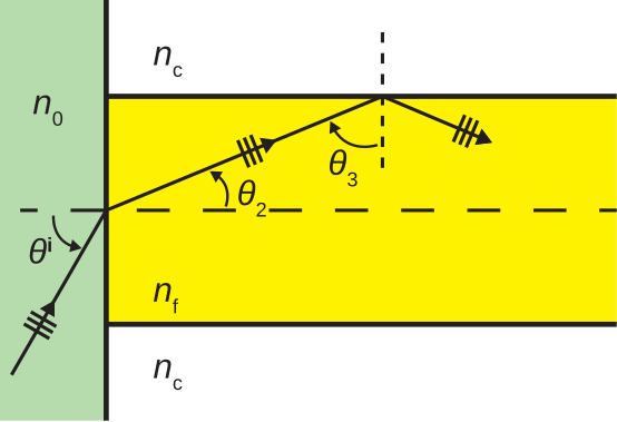
En esta figura, vemos la luz incidente de un medio que tiene índice de refracción\(n_0\), con ángulo de incidencia\(\theta^i\). La luz se transmite con ángulo de transmisión\(\theta_2\) a la fibra, y posteriormente incide sobre la superficie del revestimiento con ángulo de incidencia\(\theta_3\). Para que la luz se propague sin pérdida dentro del cable, se requiere que
\[\sin\theta_3 \ge \frac{n_c}{n_f} \label{m0192_eCAnm} \]
ya que este criterio debe cumplirse para que se produzca una reflexión interna total.
Ahora considere la restricción que la Ecuación\ ref {M0192_ECANM} impone\(\theta^i\). En primer lugar, observamos que\(\theta_3\) se relaciona con\(\theta_2\) lo siguiente:
\[\theta_3 = \frac{\pi}{2} - \theta_2 \nonumber \]
por lo tanto
\ begin {align}\ sin\ theta_3 &=\ sin\ izquierda (\ frac {\ pi} {2} -\ theta_2\ derecha)\\ &=\ cos\ theta_2\ end {align}
por lo
\[\cos\theta_2 \ge \frac{n_c}{n_f} \nonumber \]
Al cuadrar ambos lados, encontramos:
\[\cos^2\theta_2 \ge \frac{n_c^2}{n_f^2} \nonumber \]
Ahora invocando una identidad trigonométrica:
\[1-\sin^2\theta_2 \ge \frac{n_c^2}{n_f^2} \nonumber \]
por lo que:
\[\sin^2\theta_2 \le 1-\frac{n_c^2}{n_f^2} \label{m0192_e1} \]
Ahora nos relacionamos con\(\theta_2\) el\(\theta^i\) uso de la ley de Snell:
\[\sin\theta_2 = \frac{n_0}{n_f}\sin\theta^i \nonumber \]
así que la Ecuación\ ref {m0192_e1} puede escribirse:
\[\frac{n_0^2}{n_f^2}\sin^2\theta^i \le 1-\frac{n_c^2}{n_f^2} \nonumber \]
Ahora resolviendo para\(\sin\theta^i\), obtenemos:
\[\sin\theta^i \le \frac{1}{n_0}\sqrt{ n_f^2 - n_c^2 } \nonumber \]
Este resultado indica el rango de ángulos de incidencia que resultan en una reflexión interna total dentro de la fibra. El valor máximo del\(\theta^i\) cual satisface esta condición se conoce como el ángulo de aceptación\(\theta_a\), por lo que:
\[\theta_a \triangleq \arcsin\left(\frac{1}{n_0}\sqrt{ n_f^2 - n_c^2 }\right) \nonumber \]
Esto lleva a la siguiente visión:
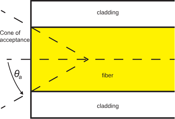
Para lanzar efectivamente luz en la fibra, es necesario que la luz llegue desde dentro de un cono que tenga medio ángulo\(\theta_a\) con respecto al eje de la fibra.
El cono de aceptación asociado se ilustra en la Figura\(\PageIndex{2}\).
También es común definir la cantidad de apertura numérica NA de la siguiente manera:
\[\mbox{NA} \triangleq \frac{1}{n_0}\sqrt{ n_f^2 - n_c^2 } \label{m0192_eNA} \]
Tenga en cuenta que\(n_0\) suele estar muy cerca de\(1\) (correspondiente a la incidencia desde el aire), por lo que es común ver NA definida como simple\(\sqrt{ n_f^2 - n_c^2 }\). Este parámetro se usa comúnmente en lugar del ángulo de aceptación en hojas de datos para cable de fibra óptica.
Los valores típicos de\(n_f\) y\(n_c\) para una fibra óptica son 1.52 y 1.49, respectivamente. ¿Cuáles son la apertura numérica y el ángulo de aceptación?
Solución
Usando la ecuación\ ref {M0192_ena} y presumiendo\(n_0=1\), encontramos NA\(\cong \underline{0.30}\). Desde\(\sin\theta_a =\) NA, nos encontramos\(\theta_a=\underline{17.5^{\circ}}\). La luz debe llegar desde dentro\(17.5^{\circ}\) desde el eje de la fibra para asegurar una reflexión interna total dentro de la fibra.