
1.2: Características del pulso
- Page ID
- 84957
\( \newcommand{\vecs}[1]{\overset { \scriptstyle \rightharpoonup} {\mathbf{#1}} } \)
\( \newcommand{\vecd}[1]{\overset{-\!-\!\rightharpoonup}{\vphantom{a}\smash {#1}}} \)
\( \newcommand{\dsum}{\displaystyle\sum\limits} \)
\( \newcommand{\dint}{\displaystyle\int\limits} \)
\( \newcommand{\dlim}{\displaystyle\lim\limits} \)
\( \newcommand{\id}{\mathrm{id}}\) \( \newcommand{\Span}{\mathrm{span}}\)
( \newcommand{\kernel}{\mathrm{null}\,}\) \( \newcommand{\range}{\mathrm{range}\,}\)
\( \newcommand{\RealPart}{\mathrm{Re}}\) \( \newcommand{\ImaginaryPart}{\mathrm{Im}}\)
\( \newcommand{\Argument}{\mathrm{Arg}}\) \( \newcommand{\norm}[1]{\| #1 \|}\)
\( \newcommand{\inner}[2]{\langle #1, #2 \rangle}\)
\( \newcommand{\Span}{\mathrm{span}}\)
\( \newcommand{\id}{\mathrm{id}}\)
\( \newcommand{\Span}{\mathrm{span}}\)
\( \newcommand{\kernel}{\mathrm{null}\,}\)
\( \newcommand{\range}{\mathrm{range}\,}\)
\( \newcommand{\RealPart}{\mathrm{Re}}\)
\( \newcommand{\ImaginaryPart}{\mathrm{Im}}\)
\( \newcommand{\Argument}{\mathrm{Arg}}\)
\( \newcommand{\norm}[1]{\| #1 \|}\)
\( \newcommand{\inner}[2]{\langle #1, #2 \rangle}\)
\( \newcommand{\Span}{\mathrm{span}}\) \( \newcommand{\AA}{\unicode[.8,0]{x212B}}\)
\( \newcommand{\vectorA}[1]{\vec{#1}} % arrow\)
\( \newcommand{\vectorAt}[1]{\vec{\text{#1}}} % arrow\)
\( \newcommand{\vectorB}[1]{\overset { \scriptstyle \rightharpoonup} {\mathbf{#1}} } \)
\( \newcommand{\vectorC}[1]{\textbf{#1}} \)
\( \newcommand{\vectorD}[1]{\overrightarrow{#1}} \)
\( \newcommand{\vectorDt}[1]{\overrightarrow{\text{#1}}} \)
\( \newcommand{\vectE}[1]{\overset{-\!-\!\rightharpoonup}{\vphantom{a}\smash{\mathbf {#1}}}} \)
\( \newcommand{\vecs}[1]{\overset { \scriptstyle \rightharpoonup} {\mathbf{#1}} } \)
\(\newcommand{\longvect}{\overrightarrow}\)
\( \newcommand{\vecd}[1]{\overset{-\!-\!\rightharpoonup}{\vphantom{a}\smash {#1}}} \)
\(\newcommand{\avec}{\mathbf a}\) \(\newcommand{\bvec}{\mathbf b}\) \(\newcommand{\cvec}{\mathbf c}\) \(\newcommand{\dvec}{\mathbf d}\) \(\newcommand{\dtil}{\widetilde{\mathbf d}}\) \(\newcommand{\evec}{\mathbf e}\) \(\newcommand{\fvec}{\mathbf f}\) \(\newcommand{\nvec}{\mathbf n}\) \(\newcommand{\pvec}{\mathbf p}\) \(\newcommand{\qvec}{\mathbf q}\) \(\newcommand{\svec}{\mathbf s}\) \(\newcommand{\tvec}{\mathbf t}\) \(\newcommand{\uvec}{\mathbf u}\) \(\newcommand{\vvec}{\mathbf v}\) \(\newcommand{\wvec}{\mathbf w}\) \(\newcommand{\xvec}{\mathbf x}\) \(\newcommand{\yvec}{\mathbf y}\) \(\newcommand{\zvec}{\mathbf z}\) \(\newcommand{\rvec}{\mathbf r}\) \(\newcommand{\mvec}{\mathbf m}\) \(\newcommand{\zerovec}{\mathbf 0}\) \(\newcommand{\onevec}{\mathbf 1}\) \(\newcommand{\real}{\mathbb R}\) \(\newcommand{\twovec}[2]{\left[\begin{array}{r}#1 \\ #2 \end{array}\right]}\) \(\newcommand{\ctwovec}[2]{\left[\begin{array}{c}#1 \\ #2 \end{array}\right]}\) \(\newcommand{\threevec}[3]{\left[\begin{array}{r}#1 \\ #2 \\ #3 \end{array}\right]}\) \(\newcommand{\cthreevec}[3]{\left[\begin{array}{c}#1 \\ #2 \\ #3 \end{array}\right]}\) \(\newcommand{\fourvec}[4]{\left[\begin{array}{r}#1 \\ #2 \\ #3 \\ #4 \end{array}\right]}\) \(\newcommand{\cfourvec}[4]{\left[\begin{array}{c}#1 \\ #2 \\ #3 \\ #4 \end{array}\right]}\) \(\newcommand{\fivevec}[5]{\left[\begin{array}{r}#1 \\ #2 \\ #3 \\ #4 \\ #5 \\ \end{array}\right]}\) \(\newcommand{\cfivevec}[5]{\left[\begin{array}{c}#1 \\ #2 \\ #3 \\ #4 \\ #5 \\ \end{array}\right]}\) \(\newcommand{\mattwo}[4]{\left[\begin{array}{rr}#1 \amp #2 \\ #3 \amp #4 \\ \end{array}\right]}\) \(\newcommand{\laspan}[1]{\text{Span}\{#1\}}\) \(\newcommand{\bcal}{\cal B}\) \(\newcommand{\ccal}{\cal C}\) \(\newcommand{\scal}{\cal S}\) \(\newcommand{\wcal}{\cal W}\) \(\newcommand{\ecal}{\cal E}\) \(\newcommand{\coords}[2]{\left\{#1\right\}_{#2}}\) \(\newcommand{\gray}[1]{\color{gray}{#1}}\) \(\newcommand{\lgray}[1]{\color{lightgray}{#1}}\) \(\newcommand{\rank}{\operatorname{rank}}\) \(\newcommand{\row}{\text{Row}}\) \(\newcommand{\col}{\text{Col}}\) \(\renewcommand{\row}{\text{Row}}\) \(\newcommand{\nul}{\text{Nul}}\) \(\newcommand{\var}{\text{Var}}\) \(\newcommand{\corr}{\text{corr}}\) \(\newcommand{\len}[1]{\left|#1\right|}\) \(\newcommand{\bbar}{\overline{\bvec}}\) \(\newcommand{\bhat}{\widehat{\bvec}}\) \(\newcommand{\bperp}{\bvec^\perp}\) \(\newcommand{\xhat}{\widehat{\xvec}}\) \(\newcommand{\vhat}{\widehat{\vvec}}\) \(\newcommand{\uhat}{\widehat{\uvec}}\) \(\newcommand{\what}{\widehat{\wvec}}\) \(\newcommand{\Sighat}{\widehat{\Sigma}}\) \(\newcommand{\lt}{<}\) \(\newcommand{\gt}{>}\) \(\newcommand{\amp}{&}\) \(\definecolor{fillinmathshade}{gray}{0.9}\)La mayoría de las veces, no hay un pulso aislado, sino un tren de pulsos.
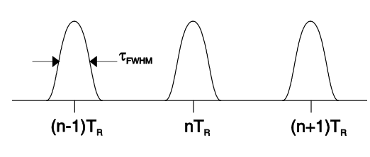
\(T_R\): tiempo de repetición de pulso
\(W\): energía de pulso
\(P_{ave} = W/T_R\): la potencia promedio
\(\tau{\text{FWHM}}\) es la anchura completa a la mitad máxima de la envolvente de intensidad del pulso en el dominio del tiempo.
La potencia máxima viene dada por
\[P_p = \dfrac{W}{\tau{\text{FWHM}}} = P_{ave} \dfrac{T_R}{\tau{\text{FWHM}}} \nonumber \]
y el campo eléctrico pico viene dado por
\[E_p = \sqrt{2 Z_{F_0} \dfrac{P_p}{A_{\text{eff}}} \nonumber \]
\(A_{\text{eff}}\)es la sección transversal del haz y\(Z_{F_0} = 377 \Omega\) es la impedancia del espacio libre.
Escalas de tiempo:
\[\begin{array} {lcl} {\text{1 ns}} & \sim & {30\text{ cm (high-speed electronics, GHz}} \\ {\text{1 ps}} & \sim & {300\ \mu\text{m}} \\ {\text{1 fs}} & \sim & {\text{300 nm}} \\ {1 \text{ as} = 10^{-18} s} & \sim & {\text{0.3 nm = 3} \mathring{A} \text{ (typ-lattice constant in metal)}} \end{array} \nonumber \]
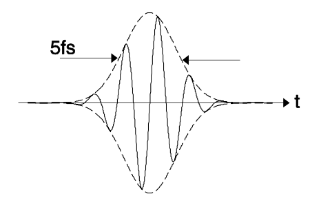
Los pulsos más cortos generados hasta la fecha son aproximadamente 4 - 5 fs a 800 nm\((\lambda/c = 2.7\) fs), menos de dos ciclos ópticos y 250 como a 25 nm. Para pulsos de algunos ciclos, el campo eléctrico se vuelve importante, ¡no solo la intensidad!
potencia media:
\[\begin{array} {cl} {P_{ave} \sim} & {\text{1W, up to 100 W in progress.}} \\ {\ } & {\text{kW possible, not yet pulsed}} \end{array} \nonumber \]
tasas de repetición:
\[T_R^{-1} = f_R = \text{m Hz - 100 GHz}\nonumber \]
energía de pulso:
\[W = 1pJ - 1kJ\nonumber \]
ancho de pulso:
\[\tau_{\text{FWHM}} = \begin{array} {ll} {\text{5 fs - 50 ps,}} & {\text{modelocked}} \\ {\text{30 ps - 100 ns,}} & {\text{Q - switched}} \end{array}\nonumber \]
potencia pico:
\[P_p = \dfrac{\text{1 kJ}}{\text{1 ps}} \sim \text{1 PW},\nonumber \]
obtenido con Nd:vidrio (LLNL - USA, [1] [2] [3]).
Para un pulso de laboratorio típico, la potencia máxima es
\[P_p = \dfrac{\text{10 nJ}}{\text{10 fs}} \sim \text{1 MW}\nonumber \]
campo pico del pulso típico de laboratorio:
\[E_p = \sqrt{2 \times 377 \times \dfrac{10^6 \times 10^{12}}{\pi \times (1.5)^2}} \dfrac{\text{V}}{\text{m}} \approx 10^{10} \dfrac{\text{V}}{\text{m}} = \dfrac{10\text{V}}{\text{nm}}\nonumber \]