
3.1: Introducción a los procesos de media móvil autorregresiva (ARMA)
- Page ID
- 148662

En este capítulo se discuten procesos de media móvil autorregresiva. Desempeñan un papel crucial en la especificación de modelos de series de tiempo para aplicaciones. Como las soluciones de ecuaciones de diferencia estocástica con coeficientes constantes y estos procesos poseen una estructura lineal.
Definición 3.1.1: Procesos ARMA
(a) Un proceso débilmente estacionario\(X_t\colon t\in\mathbb{Z}\) se denomina serie de tiempo de promedio móvil autorregresivo de orden\(p,q\), abreviado por\(ARMA(p,q)\), si satisface las ecuaciones de diferencia
\ [\ begin {ecuación}\ label {eq:3.1.1}
x_t=\ phi_1x_ {t-1} +\ ldots+\ pHI_px_ {t-p} +z_t+\ TheTa_1z_ {t-1} +\ ldots+\ TheTa_qz_ {t-q},
\ qquad
t\ in\ mathbb {Z},
\ end ecuación}\ tag {3.1.1}\]
donde\(\phi_1,\ldots,\phi_p\) y\(\theta_1,\ldots,\theta_q\) son constantes reales,\(\phi_p\not=0\not=\theta_q\), y\((Z_t\colon t\in\mathbb{Z})\sim{\rm WN}(0,\sigma^2)\).
(b) Un proceso estocástico débilmente estacionario\(X_t\colon t\in\mathbb{Z}\) se denomina serie\(ARMA(p,q)\) temporal con media\(\mu\) si el proceso\(X_t-\mu\colon t\in\mathbb{Z}\) satisface el sistema de ecuaciones.
Se puede obtener una representación más concisa de la Ecuación\ ref {eq:3.1.1} con el uso del operador de retroceso\(B\). Para ello, definir el polinomio autorregresivo y el polinomio promedio móvil por
\[ \phi(z)=1-\phi_1z-\phi_2z^2-\ldots-\phi_pz^p,\qquad z\in\mathbb{C}, \nonumber \]
y
\[ \theta(z)=1+\theta_1z+\theta_2z^2+\ldots+\theta_qz^q,\qquad z\in\mathbb{C}, \nonumber \]
respectivamente, donde\(\mathbb{C}\) denota el conjunto de números complejos. Insertando el operador de retroceso en estos polinomios, las ecuaciones en (3.1.1) se convierten en
\ [\ begin {ecuación}\ label {eq:3.1.2}
\ phi (B) x_t=\ theta (B) z_t,\ qquad t\ in\ mathbb {Z}.
\ end {ecuación}\ tag {3.1.2}\]
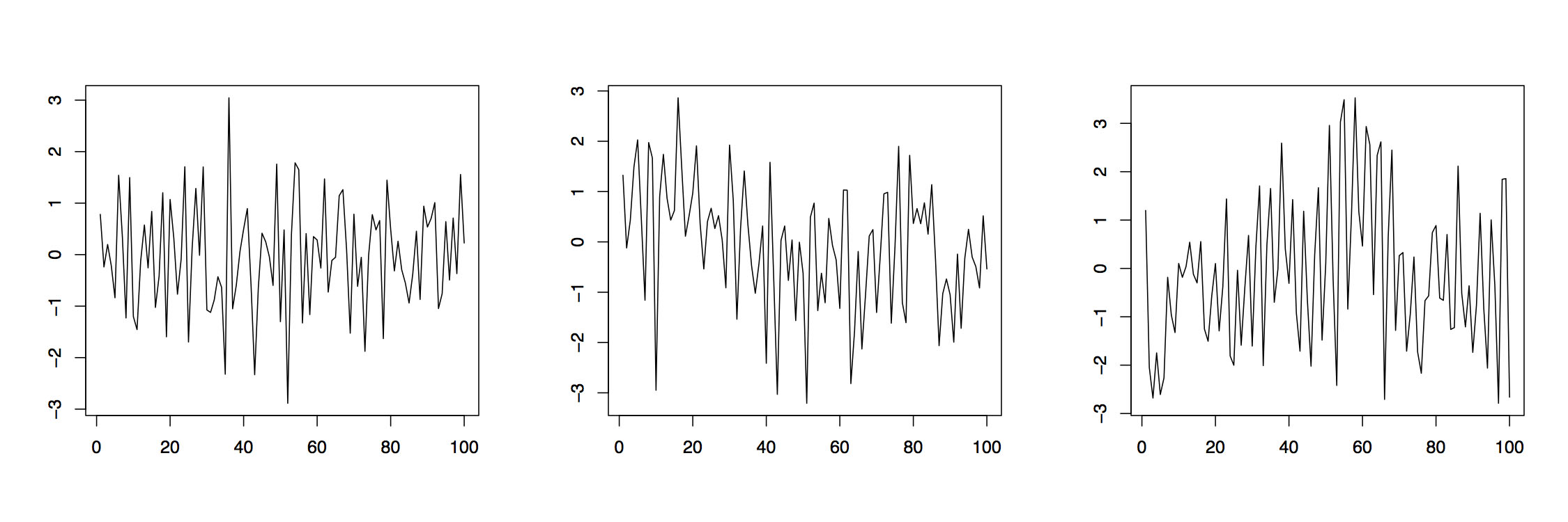
Ejemplo 3.1.1 La Figura 3.1 muestra realizaciones de tres series de tiempo promedio móvil autorregresivas diferentes basadas en series de tiempo independientes, estándar distribuidas normalmente\((Z_t\colon t\in\mathbb{Z})\). The left panel is an ARMA(2,2) process with parameter specifications \(\phi_1=.2\), \(\phi_2=-.3\), \(\theta_1=-.5\) and \(\theta_2=.3\). The middle plot is obtained from an ARMA(1,4) process with parameters \(\phi_1=.3\), \(\theta_1=-.2\), \(\theta_2=-.3\), \(\theta_3=.5\), and \(\theta_4=.2\), while the right plot is from an ARMA(4,1) with parameters \(\phi_1=-.2\), \(\phi_2=-.3\), \(\phi_3=.5\) and \(\phi_4=.2\) and \(\theta_1=.6\). The plots indicate that ARMA models can provide a flexible tool for modeling diverse residual sequences. It will turn out in the next section that all three realizations here come from (strictly) stationary processes. Similar time series plots can be produced in R using the commands
>arima22 =
arima.sim (lista (orden=c (2,0,2), ar=c (.2, -.3), ma=c (-.5, .3)), n=100)
>arima14 =
arima.sim (lista (orden=c (1,0,4), ar=.3, ma=c (-.2, -.3, .5, .2)), n=100)
>arima41 =
arima.sim (lista (orden=c (4,0,1), ar=c (-.2, -.3, .5, .2), ma=.6), n= 100)
Algunos casos especiales cubiertos en los siguientes dos ejemplos tienen particular relevancia en el análisis de series temporales.
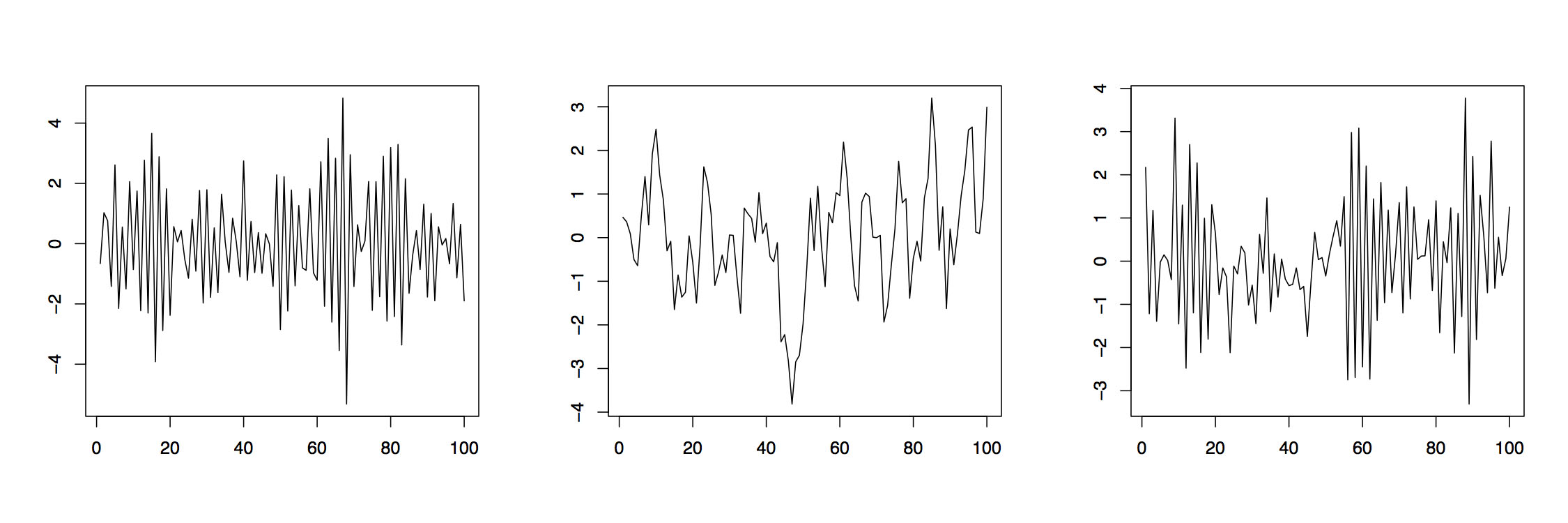
Ejemplo 3.1.2 (Procesos AR) Si el polinomio promedio móvil en (3.1.2) es igual a uno, es decir, si\(\theta(z)\equiv 1\), then the resulting \((X_t\colon t\in\mathbb{Z})\)is referred to as autoregressive process of order \(p\), AR\((p)\). These time series interpret the value of the current variable \(X_t\) as a linear combination of \(p\) previous variables \(X_{t-1},\ldots,X_{t-p}\) plus an additional distortion by the white noise \(Z_t\). Figure 3.1.2 displays two AR(1) processes with respective parameters \(\phi_1=-.9\) (left) and \(\phi_1=.8\) (middle) as well as an AR(2) process with parameters \(\phi_1=-.5\) and \(\phi_2=.3\). The corresponding R commands are
>ar1neg = arima.sim (lista (orden=c (1,0,0), ar=-.9), n=100)
>ar1pos = arima.sim (lista (orden=c (1,0,0), ar=.8), n=100)
>ar2 = arima.sim (lista (pedido=c (2,0,0), ar=c (-.5, .3)), n=100)
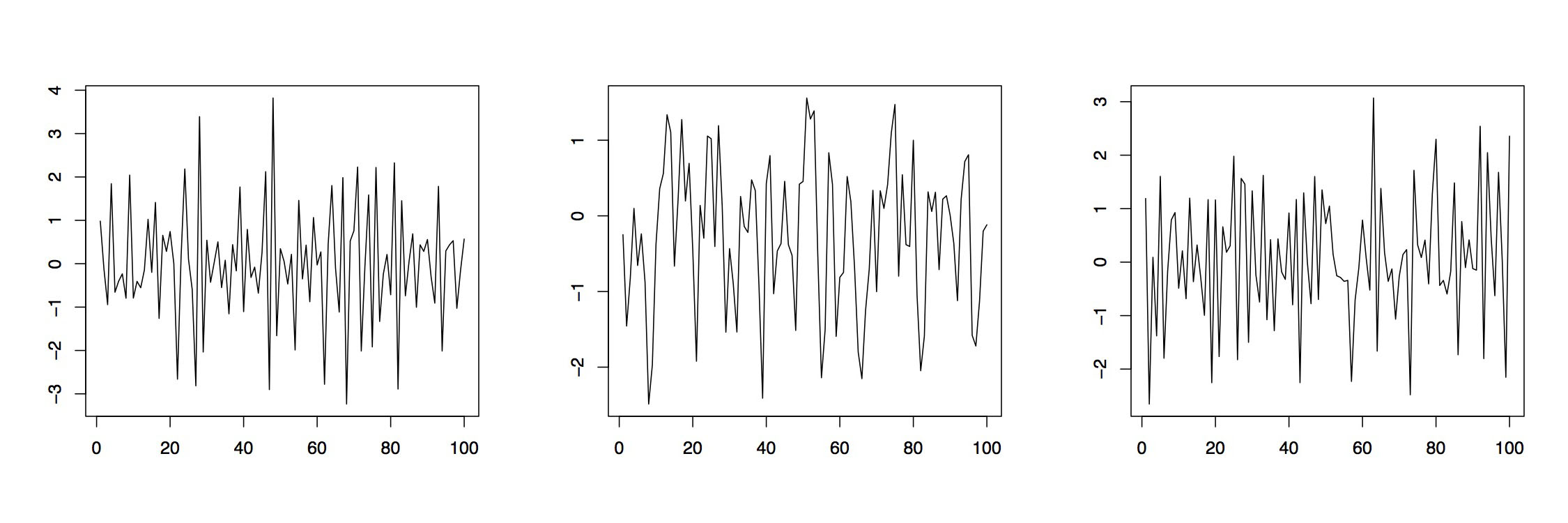
Figura 3.3: Realización de tres procesos de media móvil.
Ejemplo 3.1.3 (Procesos MA) Si el polinomio autorregresivo en (3.1.2) es igual a uno, es decir, si\(\phi(z)\equiv 1\), then the resulting \((X_t\colon t\in\mathbb{Z})\) is referred to as moving average process of order \(q\), MA(\(q\))}. Here the present variable \(X_t\) is obtained as superposition of \(q\) white noise terms \(Z_t,\ldots,Z_{t-q}\). Figure (3.1.3) shows two MA(1) processes with respective parameters \(\theta_1=.5\) (left) and \(\theta_1=-.8\) (middle). The right plot is observed from an MA(2) process with parameters \(\theta_1=-.5\) and \(\theta_2=.3\). In R one may use
> ma1pos = arima.sim (lista (pedido=c (0,0,1), ma=.5), n=100)
> ma1neg = arima.sim (lista (pedido=c (0,0,1), ma=-.8), n=100)
> ma2 = arima.sim (lista (pedido=c (0,0,2), ma=c (-.5, .3)), n=100)
Para el análisis que viene en los próximos capítulos, ahora introducimos procesos de media móvil de orden infinito\((q=\infty)\). Son una herramienta importante para determinar soluciones estacionarias a las ecuaciones de diferencia (3.1.1).
Definición 3.1.2 Procesos lineales
Un proceso estocástico\((X_t\colon t\in\mathbb{Z})\) is called linear process or MA\((\infty)\) time series if there is a sequence \((\psi_j\colon j\in\mathbb{N}_0)\) with \(\sum_{j=0}^\infty|\psi_j|<\infty\) such that
\ [\ begin {ecuación}\ label {eq:3.1.3}
x_t=\ sum_ {j=0} ^\ infty\ psi_jz_ {t-j},\ qquad t\ in\ mathbb {Z},
\ end {ecuación}\ tag {3.1.3}\]
donde\((Z_t\colon t\in\mathbb{Z})\sim{\rm WN}(0,\sigma^2)\).
Las series de tiempo promedio móviles de cualquier orden\(q\) son casos especiales de procesos lineales. Solo elige\(\psi_j=\theta_j\)\(j=1,\ldots,q\) y establece\(\psi_j=0\) si\(j>q\). Es común introducir la serie power
\[ \psi(z)=\sum_{j=0}^\infty\psi_jz^j, \qquad z\in\mathbb{C}, \nonumber \]
para expresar un proceso lineal en términos del operador de retroceso. La pantalla (3.1.3) ahora se puede reescribir en forma compacta
\[ X_t=\psi(B)Z_t,\qquad t\in\mathbb{Z}. \nonumber \]
Con las definiciones de esta sección a la mano, las propiedades de los procesos ARMA, como la estacionariedad e invertibilidad, se investigan en la siguiente sección. La sección actual se cierra dando sentido a la notación\(X_t=\psi(B)Z_t\). Note that one is possibly dealing with an infinite sum of random variables. For completeness and later use, in the following example the mean and ACVF of a linear process are derived.
Ejemplo 3.1.4 Media y ACVF de un proceso lineal
Dejar\((X_t\colon t\in\mathbb{Z})\) ser un proceso lineal de acuerdo a la Definición 3.1.2. Entonces, sostiene que
\[ E[X_t] =E\left[\sum_{j=0}^\infty\psi_jZ_{t-j}\right] =\sum_{j=0}^\infty\psi_jE[Z_{t-j}]=0, \qquad t\in\mathbb{Z}. \nonumber \]
Siguiente observar también que
\ begin {align*}
\ gamma (h)
&=\ mathrm {Cov} (X_ {t+h}, x_t)\\ [.2cm]
&=E\ left [\ sum_ {j=0} ^\ infty\ psi_jz_ {t+h-j}\ sum_ {k=0} ^\ infty\ psi_kz_ {t-j k}\ derecha]\\ [.2cm]
&=\ sigma^2\ suma_ {k=0} ^\ infty\ psi_ {k+h}\ psi_k<\ infty
\ end {align*}
por suposición sobre la secuencia\((\psi_j\colon j\in\mathbb{N}_0)\).