
1.8: Flujo
- Page ID
- 131769

\( \newcommand{\vecs}[1]{\overset { \scriptstyle \rightharpoonup} {\mathbf{#1}} } \)
\( \newcommand{\vecd}[1]{\overset{-\!-\!\rightharpoonup}{\vphantom{a}\smash {#1}}} \)
\( \newcommand{\dsum}{\displaystyle\sum\limits} \)
\( \newcommand{\dint}{\displaystyle\int\limits} \)
\( \newcommand{\dlim}{\displaystyle\lim\limits} \)
\( \newcommand{\id}{\mathrm{id}}\) \( \newcommand{\Span}{\mathrm{span}}\)
( \newcommand{\kernel}{\mathrm{null}\,}\) \( \newcommand{\range}{\mathrm{range}\,}\)
\( \newcommand{\RealPart}{\mathrm{Re}}\) \( \newcommand{\ImaginaryPart}{\mathrm{Im}}\)
\( \newcommand{\Argument}{\mathrm{Arg}}\) \( \newcommand{\norm}[1]{\| #1 \|}\)
\( \newcommand{\inner}[2]{\langle #1, #2 \rangle}\)
\( \newcommand{\Span}{\mathrm{span}}\)
\( \newcommand{\id}{\mathrm{id}}\)
\( \newcommand{\Span}{\mathrm{span}}\)
\( \newcommand{\kernel}{\mathrm{null}\,}\)
\( \newcommand{\range}{\mathrm{range}\,}\)
\( \newcommand{\RealPart}{\mathrm{Re}}\)
\( \newcommand{\ImaginaryPart}{\mathrm{Im}}\)
\( \newcommand{\Argument}{\mathrm{Arg}}\)
\( \newcommand{\norm}[1]{\| #1 \|}\)
\( \newcommand{\inner}[2]{\langle #1, #2 \rangle}\)
\( \newcommand{\Span}{\mathrm{span}}\) \( \newcommand{\AA}{\unicode[.8,0]{x212B}}\)
\( \newcommand{\vectorA}[1]{\vec{#1}} % arrow\)
\( \newcommand{\vectorAt}[1]{\vec{\text{#1}}} % arrow\)
\( \newcommand{\vectorB}[1]{\overset { \scriptstyle \rightharpoonup} {\mathbf{#1}} } \)
\( \newcommand{\vectorC}[1]{\textbf{#1}} \)
\( \newcommand{\vectorD}[1]{\overrightarrow{#1}} \)
\( \newcommand{\vectorDt}[1]{\overrightarrow{\text{#1}}} \)
\( \newcommand{\vectE}[1]{\overset{-\!-\!\rightharpoonup}{\vphantom{a}\smash{\mathbf {#1}}}} \)
\( \newcommand{\vecs}[1]{\overset { \scriptstyle \rightharpoonup} {\mathbf{#1}} } \)
\(\newcommand{\longvect}{\overrightarrow}\)
\( \newcommand{\vecd}[1]{\overset{-\!-\!\rightharpoonup}{\vphantom{a}\smash {#1}}} \)
\(\newcommand{\avec}{\mathbf a}\) \(\newcommand{\bvec}{\mathbf b}\) \(\newcommand{\cvec}{\mathbf c}\) \(\newcommand{\dvec}{\mathbf d}\) \(\newcommand{\dtil}{\widetilde{\mathbf d}}\) \(\newcommand{\evec}{\mathbf e}\) \(\newcommand{\fvec}{\mathbf f}\) \(\newcommand{\nvec}{\mathbf n}\) \(\newcommand{\pvec}{\mathbf p}\) \(\newcommand{\qvec}{\mathbf q}\) \(\newcommand{\svec}{\mathbf s}\) \(\newcommand{\tvec}{\mathbf t}\) \(\newcommand{\uvec}{\mathbf u}\) \(\newcommand{\vvec}{\mathbf v}\) \(\newcommand{\wvec}{\mathbf w}\) \(\newcommand{\xvec}{\mathbf x}\) \(\newcommand{\yvec}{\mathbf y}\) \(\newcommand{\zvec}{\mathbf z}\) \(\newcommand{\rvec}{\mathbf r}\) \(\newcommand{\mvec}{\mathbf m}\) \(\newcommand{\zerovec}{\mathbf 0}\) \(\newcommand{\onevec}{\mathbf 1}\) \(\newcommand{\real}{\mathbb R}\) \(\newcommand{\twovec}[2]{\left[\begin{array}{r}#1 \\ #2 \end{array}\right]}\) \(\newcommand{\ctwovec}[2]{\left[\begin{array}{c}#1 \\ #2 \end{array}\right]}\) \(\newcommand{\threevec}[3]{\left[\begin{array}{r}#1 \\ #2 \\ #3 \end{array}\right]}\) \(\newcommand{\cthreevec}[3]{\left[\begin{array}{c}#1 \\ #2 \\ #3 \end{array}\right]}\) \(\newcommand{\fourvec}[4]{\left[\begin{array}{r}#1 \\ #2 \\ #3 \\ #4 \end{array}\right]}\) \(\newcommand{\cfourvec}[4]{\left[\begin{array}{c}#1 \\ #2 \\ #3 \\ #4 \end{array}\right]}\) \(\newcommand{\fivevec}[5]{\left[\begin{array}{r}#1 \\ #2 \\ #3 \\ #4 \\ #5 \\ \end{array}\right]}\) \(\newcommand{\cfivevec}[5]{\left[\begin{array}{c}#1 \\ #2 \\ #3 \\ #4 \\ #5 \\ \end{array}\right]}\) \(\newcommand{\mattwo}[4]{\left[\begin{array}{rr}#1 \amp #2 \\ #3 \amp #4 \\ \end{array}\right]}\) \(\newcommand{\laspan}[1]{\text{Span}\{#1\}}\) \(\newcommand{\bcal}{\cal B}\) \(\newcommand{\ccal}{\cal C}\) \(\newcommand{\scal}{\cal S}\) \(\newcommand{\wcal}{\cal W}\) \(\newcommand{\ecal}{\cal E}\) \(\newcommand{\coords}[2]{\left\{#1\right\}_{#2}}\) \(\newcommand{\gray}[1]{\color{gray}{#1}}\) \(\newcommand{\lgray}[1]{\color{lightgray}{#1}}\) \(\newcommand{\rank}{\operatorname{rank}}\) \(\newcommand{\row}{\text{Row}}\) \(\newcommand{\col}{\text{Col}}\) \(\renewcommand{\row}{\text{Row}}\) \(\newcommand{\nul}{\text{Nul}}\) \(\newcommand{\var}{\text{Var}}\) \(\newcommand{\corr}{\text{corr}}\) \(\newcommand{\len}[1]{\left|#1\right|}\) \(\newcommand{\bbar}{\overline{\bvec}}\) \(\newcommand{\bhat}{\widehat{\bvec}}\) \(\newcommand{\bperp}{\bvec^\perp}\) \(\newcommand{\xhat}{\widehat{\xvec}}\) \(\newcommand{\vhat}{\widehat{\vvec}}\) \(\newcommand{\uhat}{\widehat{\uvec}}\) \(\newcommand{\what}{\widehat{\wvec}}\) \(\newcommand{\Sighat}{\widehat{\Sigma}}\) \(\newcommand{\lt}{<}\) \(\newcommand{\gt}{>}\) \(\newcommand{\amp}{&}\) \(\definecolor{fillinmathshade}{gray}{0.9}\)El producto de la intensidad del campo eléctrico y el área es el flujo\(\Phi_E\). Whereas \(E\) is an intensive quantity, \(\Phi_E\) is an extensive quantity. It dimensions are ML3T-2Q-1 and its SI units are N m2 C-1, although later on, after we have met the unit called the volt, we shall prefer to express \(\Phi_E\) in V m.
Con grados crecientes de sofisticación, el flujo puede definirse matemáticamente como:
\[\Phi_E = EA\]
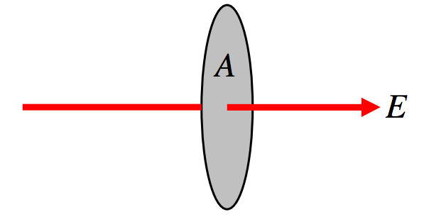
\(\text{FIGURE I.4}\): Flujo que es perpendicular a la superficie.
\[\Phi_E = EA \cos \theta = \textbf{E} \cdot \textbf{A} \]
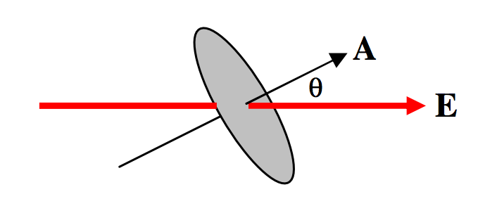
\(\text{FIGURE I.5}\): Flow that is at an angle to the surface.
Tenga en cuenta que\(\textbf{E}\) is a vector, but \(\Phi_E\) is a scalar.
\[\Phi_E = \iint \textbf{E} \cdot d\textbf{A} \]
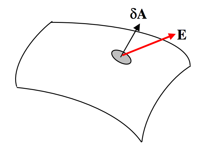
\(\text{FIGURE I.6}\)
También podemos definir un\(D\)-flux by
\[\Phi_D=\iint \textbf{D}\cdot d\textbf{A}.\]
Las dimensiones de\(\Phi_D\) are just \(Q\) and the SI units are coulombs (C).
Un ejemplo está en orden:
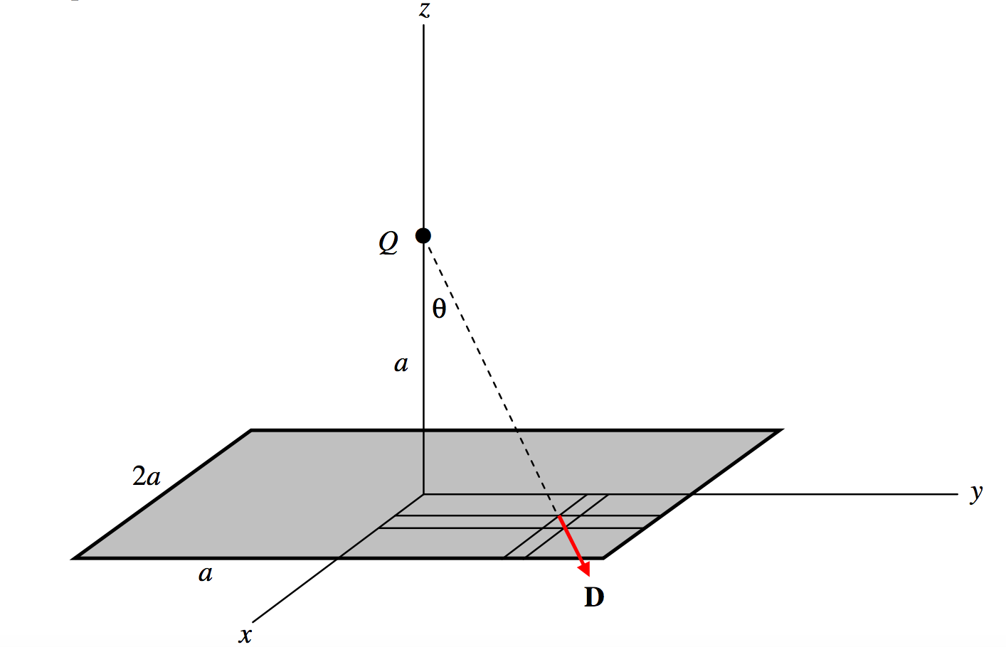
\(\text{FIGURE I.7}\)
Considera un cuadrado de lado\(2a\) in the xy-plane as shown. Suppose there is a positive charge \(Q\) at a height \(a\) on the \(z\)-axis. Calculate the total \(D\)-flux, \(\Phi_D\) through the area.
Considerar un área elemental\(dxdy\) at (\(x,\, y ,\, 0\)). Its distance from \(Q\) is \((a^2+x^2+y^2)^{1/2}\) so the magnitude of the \(D\)-field there is \(\frac{Q}{4\pi}\cdot \frac{1}{a^2+x^2+y^2}\). The scalar product of this with the area is \(\frac{Q}{4\pi}\cdot \frac{1}{a^2+x^2+y^2}\cdot \cos \theta dxdy,\text{ and }\cos \theta = \frac{a}{(a^2+x^2+y^2)^{1/2}}\). The surface integral of \(\textbf{D}\) over the whole area is
\[\label{1.8.1}\iint D\cdot dA=\frac{Qa}{\pi}\int_0^a \int_0^a \frac{dxdy}{(a^2+x^2+y^2)^{3/2}}.\]
Ahora todo lo que tenemos que hacer es la integral agradable y fácil. Let\(x=\sqrt{a^2+y^2}\tan ψ\) and the inner integral \(\int_0^a \frac{dx}{(a^2+x^2+y^2)^{3/2}}\) reduces, after some modest algebra, to \(\frac{a}{(a^2+y^2)\sqrt{2a^2+y^2}}\). Thus we now have
\[\label{1.8.2}\iint D\cdot dA = \frac{Qa^2}{\pi}\int_0^a \frac{dy}{(a^2+y^2)\sqrt{2a^2+y^2}}.\]
Con la sustitución adicional\(a^2+y^2=a^2 \sec \omega\) this reduces, after more careful algebra, to
\[\iint D\cdot dA=\frac{Q}{6}.\label{1.8.3}\]
Dos ejemplos adicionales de cálculo de integrales superficiales se pueden encontrar en la Sección 5.6, de la sección Mecánica Celestial de estas notas. Estos tratan con campos gravitacionales, pero son esencialmente los mismos que el caso electrostático; solo sustituyen\(Q\) for m and -1/(4\(\pi \epsilon\)) for \(G\).
Insto a los lectores a pasar por el dolor y el álgebra y la trigonometría de estos tres ejemplos para que puedan apreciar aún más, en la siguiente sección, el poder del teorema de Gauss.