6.5: Más sobre los motores de calor

Hasta el momento, el único motor térmico que hemos comentado con algún detalle ha sido un motor Carnot ficticio, con un gas ideal monoatómico como su gas de trabajo. Como ejemplo más realista, la figura l muestra un ciclo completo de un cilindro en un motor de automóvil estándar de combustión de gas. Este ciclo de cuatro tiempos se llama el ciclo Otto, después de su inventor, el ingeniero alemán Nikolaus Otto. El ciclo Otto es más complicado que un ciclo Carnot, de varias maneras:

• El gas de trabajo se bombea físicamente dentro y fuera del cilindro a través de válvulas, en lugar de sellarse y reutilizarse indefinidamente como en el motor Carnot.
• Los cilindros no están perfectamente aislados del bloque del motor, por lo que la energía térmica se pierde de cada cilindro por conducción. Esto hace que el motor sea menos eficiente que un motor Carnot, porque el calor se está descargando a una temperatura que no es tan fría como el ambiente.
• En lugar de calentarse por contacto con un depósito de calor externo, la mezcla aire-gas dentro de cada cilindro se calienta por combustión interna: una chispa de una bujía quema la gasolina, liberando calor.
• El gas de trabajo no es monoatómico. El aire consiste en moléculas diatómicas (\(\text{N}_2\)y\(\text{O}_2\)), y gasolina de moléculas poliatómicas como el octano (\(\text{C}_8\text{H}_{18}\)).
• El gas de trabajo no es ideal. Un gas ideal es aquel en el que las moléculas nunca interactúan entre sí, sino solo con las paredes del vaso, cuando chocan con él. En un motor de automóvil, las moléculas interactúan muy dramáticamente entre sí cuando la mezcla de aire-gas explota (y menos dramáticamente en otros momentos también, ya que, por ejemplo, la gasolina puede estar en forma de gotitas microscópicas en lugar de moléculas individuales).

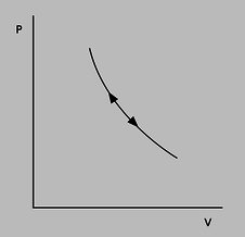
Todo esto es extremadamente complicado, y sería bueno tener alguna forma de entender y visualizar las propiedades importantes de un motor de calor de este tipo sin tratar de manejar cada detalle a la vez. Un buen método para hacer esto es un tipo de gráfico conocido como diagrama P-V. Como se demostró en el problema 2 de la tarea, la ecuación\(dW=Fdx\) para el trabajo mecánico puede ser reescrita como\(dW=PdV\) en el caso del trabajo realizado por un pistón. Aquí\(P\) representa la presión del gas de trabajo, y\(V\) su volumen. Así, en una gráfica de\(P\) versus\(V\), el área bajo la curva representa el trabajo realizado. Cuando el gas se expande,\(dx\) es positivo, y el gas hace trabajo positivo. Cuando el gas se está comprimiendo,\(dx\) es negativo, y el gas hace trabajo negativo, es decir, absorbe energía.

a / P-V diagrams for a Carnot engine and an Otto engine.

Notice how, in the diagram of the Carnot engine in the top panel of figure a, the cycle goes clockwise around the curve, and therefore the part of the curve in which negative work is being done (arrowheads pointing to the left) are below the ones in which positive work is being done. This means that over all, the engine does a positive amount of work. This net work equals the area under the top part of the curve, minus the area under the bottom part of the curve, which is simply the area enclosed by the curve. Although the diagram for the Otto engine is more complicated, we can at least compare it on the same footing with the Carnot engine. The curve forms a figure-eight, because it cuts across itself. The top loop goes clockwise, so as in the case of the Carnot engine, it represents positive work. The bottom loop goes counterclockwise, so it represents a net negative contribution to the work. This is because more work is expended in forcing out the exhaust than is generated in the intake stroke.

To make an engine as efficient as possible, we would like to make the loop have as much area as possible. What is it that determines the actual shape of the curve? First let's consider the constant-temperature expansion stroke that forms the top of the Carnot engine's P-V plot. This is analogous to the power stroke of an Otto engine. Heat is being sucked in from the hot reservoir, and since the working gas is always in thermal equilibrium with the hot reservoir, its temperature is constant. Regardless of the type of gas, we therefore have \(PV=nkT\) with \(T\) held constant, and thus \(P\propto V^{-1}\) is the mathematical shape of this curve --- a \(y=1/x\) graph, which is a hyperbola. This is all true regardless of whether the working gas is monoatomic, diatomic, or polyatomic. (The bottom of the loop is likewise of the form \(P\propto V^{-1}\), but with a smaller constant of proportionality due to the lower temperature.)

Now consider the insulated expansion stroke that forms the right side of the curve for the Carnot engine. As shown on page 324, the relationship between pressure and temperature in an insulated compression or expansion is \(T \propto P^b\), with \(b=2/5\), 2/7, or 1/4, respectively, for a monoatomic, diatomic, or polyatomic gas. For \(P\) as a function of \(V\) at constant \(T\), the ideal gas law gives \(P\propto T/V\), so \(P\propto V^{-\gamma}\), where \(\gamma=1/(1-b)\) takes on the values 5/3, 7/5, and 4/3. The number \(\gamma\) can be interpreted as the ratio \(C_P/C_V\), where \(C_P\), the heat capacity at constant pressure, is the amount of heat required to raise the temperature of the gas by one degree while keeping its pressure constant, and \(C_V\) is the corresponding quantity under conditions of constant volume.

Example 22: The compression ratio

Operating along a constant-temperature stroke, the amount of mechanical work done by a heat engine can be calculated as follows: \[\begin{align*} PV &= nkT \\ \text{Setting $c=nkT$ to simplify the writing,} P &= cV^{-1} \\ W &= \int_{V_i}^{V_f} P dV \\ &= c \int_{V_i}^{V_f} V^{-1} dV \\ &= c \ln V_f - c \ln V_i \\ &= c \ln (V_f/V_i) \end{align*}\] The ratio \(V_f/V_i\) is called the compression ratio of the engine, and higher values result in more power along this stroke. Along an insulated stroke, we have \(P\propto V^{-\gamma}\), with \(\gamma\ne1\), so the result for the work no longer has this perfect mathematical property of depending only on the ratio \(V_f/V_i\). Nevertheless, the compression ratio is still a good figure of merit for predicting the performance of any heat engine, including an internal combustion engine. High compression ratios tend to make the working gas of an internal combustion engine heat up so much that it spontaneously explodes. When this happens in an Otto-cycle engine, it can cause ignition before the sparkplug fires, an undesirable effect known as pinging. For this reason, the compression ratio of an Otto-cycle automobile engine cannot normally exceed about 10. In a diesel engine, however, this effect is used intentionally, as an alternative to sparkplugs, and compression ratios can be 20 or more.

Example 23: Sound

b / Example 23. Figure b shows a P-V plot for a sound wave. As the pressure oscillates up and down, the air is heated and cooled by its compression and expansion. Heat conduction is a relatively slow process, so typically there is not enough time over each cycle for any significant amount of heat to flow from the hot areas to the cold areas. (This is analogous to insulated compression or expansion of a heat engine; in general, a compression or expansion of this type, with no transfer of heat, is called adiabatic.) The pressure and volume of a particular little piece of the air are therefore related according to \(P\propto V^{-\gamma}\). The cycle of oscillation consists of motion back and forth along a single curve in the P-V plane, and since this curve encloses zero volume, no mechanical work is being done: the wave (under the assumed ideal conditions) propagates without any loss of energy due to friction. The speed of sound is also related to \(\gamma\). See example 13 on p. 375.

Example 24: Measuring \(\gamma\) using the “spring of air”

c / Example 24. Figure c shows an experiment that can be used to measure the \(\gamma\) of a gas. When the mass \(m\) is inserted into bottle's neck, which has cross-sectional area \(A\), the mass drops until it compresses the air enough so that the pressure is enough to support its weight. The observed frequency \(\omega\) of oscillations about this equilibrium position \(y_\text{o}\) can be used to extract the \(\gamma\) of the gas. \[\begin{align*} \omega^2 &= \frac{k}{m} \\ &= \left.-\frac{1}{m}\:\frac{dF}{dy}\right|_{y_\text{o}} \\ &= \left.-\frac{A}{m}\:\frac{dP}{dy}\right|_{y_\text{o}} \\ &= \left.-\frac{A^2}{m}\:\frac{dP}{dV}\right|_{V_\text{o}} \end{align*}\] We make the bottle big enough so that its large surface-to-volume ratio prevents the conduction of any significant amount of heat through its walls during one cycle, so \(P\propto V^{-\gamma}\), and \(dP/dV=-\gamma P/V\). Thus, \[\begin{align*} \omega^2 &= \gamma\frac{A^2}{m}\:\frac{P_\text{o}}{V_\text{o}} \end{align*}\]

Example 25: The Helmholtz resonator

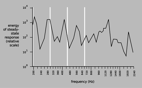
When you blow over the top of a beer bottle, you produce a pure tone. As you drink more of the beer, the pitch goes down. This is similar to example 24, except that instead of a solid mass \(m\) sitting inside the neck of the bottle, the moving mass is the air itself. As air rushes in and out of the bottle, its velocity is highest at the bottleneck, and since kinetic energy is proportional to the square of the velocity, essentially all of the kinetic energy is that of the air that's in the neck. In other words, we can replace \(m\) with \(AL\rho\), where \(L\) is the length of the neck, and \(\rho\) is the density of the air. Substituting into the earlier result, we find that the resonant frequency is \[\begin{align*} \omega^2 &= \gamma\frac{P_\text{o}}{\rho}\:\frac{A}{LV_\text{o}} . \end{align*}\] This is known as a Helmholtz resonator. As shown in figure d, a violin or an acoustic guitar has a Helmholtz resonance, since air can move in and out through the f-holes. Problem 10 is a more quantitative exploration of this. d / The resonance curve of a 1713 Stradivarius violin, measured by Carleen Hutchins. There are a number of different resonance peaks, some strong and some weak; the ones near 200 and 400 Hz are vibrations of the wood, but the one near 300 Hz is a resonance of the air moving in and out through those holes shaped like the letter F. The white lines show the frequencies of the four strings.

We have already seen, based on the microscopic nature of entropy, that any Carnot engine has the same efficiency, and the argument only employed the assumption that the engine met the definition of a Carnot cycle: two insulated strokes, and two constant-temperature strokes. Since we didn't have to make any assumptions about the nature of the working gas being used, the result is evidently true for diatomic or polyatomic molecules, or for a gas that is not ideal. This result is surprisingly simple and general, and a little mysterious --- it even applies to possibilities that we have not even considered, such as a Carnot engine designed so that the working “gas” actually consists of a mixture of liquid droplets and vapor, as in a steam engine. How can it always turn out so simple, given the kind of mathematical complications that were swept under the rug in example 22? A better way to understand this result is by switching from P-V diagrams to a diagram of temperature versus entropy, as shown in figure e.

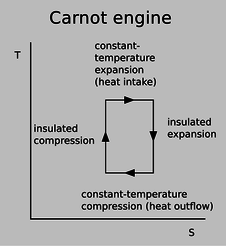
e / A T-S diagram for a Carnot engine.

An infinitesimal transfer of heat \(dQ\) gives rise to a change in entropy \(dS=dQ/T\), so the area under the curve on a T-S plot gives the amount of heat transferred. The area under the top edge of the box in figure e, extending all the way down to the axis, represents the amount of heat absorbed from the hot reservoir, while the smaller area under the bottom edge represents the heat wasted into the cold reservoir. By conservation of energy, the area enclosed by the box therefore represents the amount of mechanical work being done, as for a P-V diagram. We can now see why the efficiency of a Carnot engine is independent of any of the physical details: the definition of a Carnot engine guarantees that the T-S diagram will be a rectangular box, and the efficiency depends only on the relative heights of the top and bottom of the box.

Contributors and Attributions

Template:ContribCrowell